Classification

Logistic Regression

The classification problem is different from the regression problem in that $y$ takes a discrete value (a category label) rather than a continuous value.

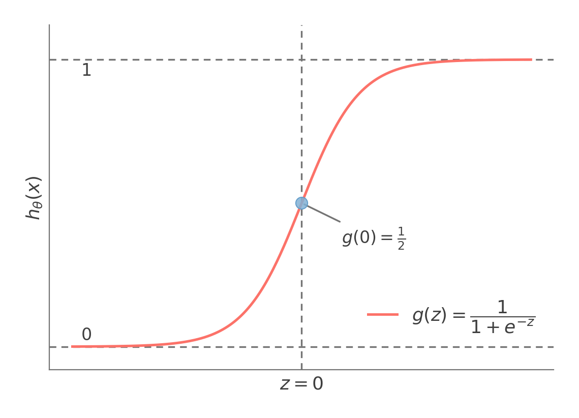
Therefore, for logistic regression, we will choose our $h_{\theta}(x)$ to be a sigmoid function that squishes any real number to a value between 0 and 1.

h_{\theta}(x) = g(\theta^T x) = \frac{1}{1 + e^{-\theta^T x}}

Sigmoid curve mapping real-valued scores to probabilities between 0 and 1 — The sigmoid function converts the score $\theta^T x$ into a probability, with $g(0) = \frac{1}{2}$ .

Let's assume that:

p(y=1 ; x, \theta) = h_{\theta}(x)

p(y=0 ; x, \theta) = 1 - h_{\theta}(x)

Now this can be rewritten as:

p(y \mid x, \theta) = (h_{\theta}(x))^y (1 - h_{\theta}(x))^{1 - y}

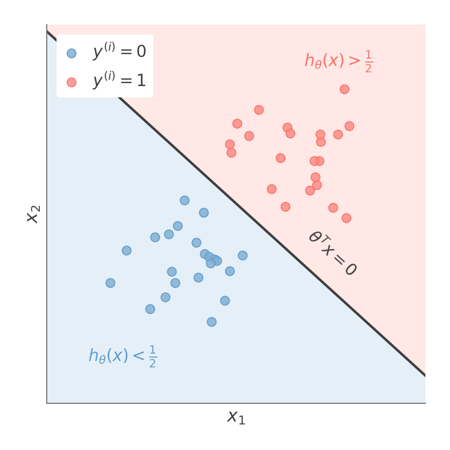
Binary classification decision boundary separating two classes — Logistic regression predicts one class on one side of the boundary $\theta^T x = 0$ and the other class on the opposite side.

Now, the log-likelihood can be written as:

\ell(\theta) = \log \, \prod_{i=1}^n \, p(y^{(i)} \mid x^{(i)}, \theta)

= \sum_{i=1}^n \, \log \, p(y^{(i)} \mid x^{(i)}, \theta)

= \sum_{i=1}^n \, \log \, \left[\left(h_{\theta}(x^{(i)})\right)^{y^{(i)}} \left(1 - h_{\theta}(x^{(i)})\right)^{1 - y^{(i)}} \right]

Taking its derivative with respect to $\theta$ , we get:

\frac{\partial}{\partial \theta_j} \, \ell(\theta) = \sum_{i=1}^n \left(y^{(i)} - h_{\theta}(x^{(i)}) \right) x_j^{(i)}

And so our gradient descent update rule to maximize the log-likelihood becomes:

\theta_j \leftarrow \theta_j + \alpha \left(y^{(i)} - h_{\theta}(x^{(i)}) \right) x_j^{(i)}

See derivation

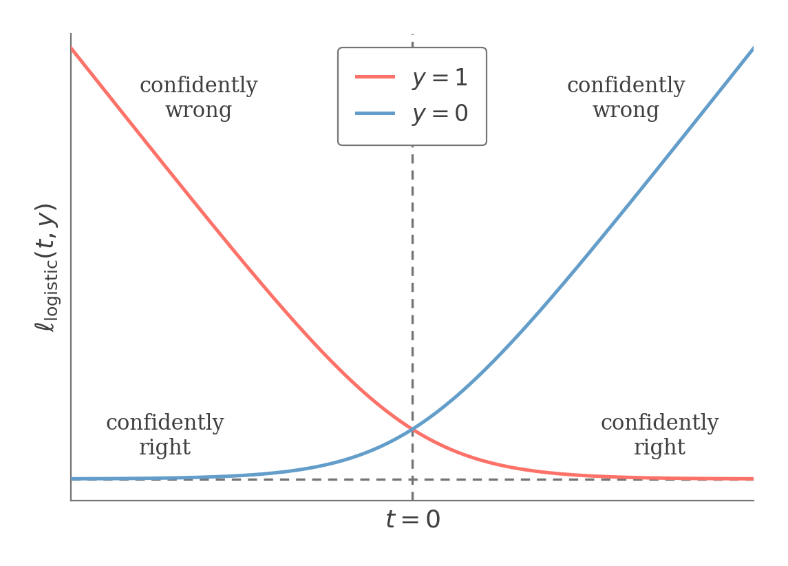
Also, note that maximizing the log-likelihood is equivalent to minimizing the logistic loss where $t = \theta^T x$

\arg \min_{\theta} \ell_{logistic}(t, y) = \arg \max_{\theta} \ell(\theta)

Logistic loss as a function of the score for each label — Minimizing the logistic loss pushes the score $t = \theta^T x$ toward the correct sign: a confidently wrong prediction is penalized without bound, while a confidently correct one costs almost nothing.

See derivation

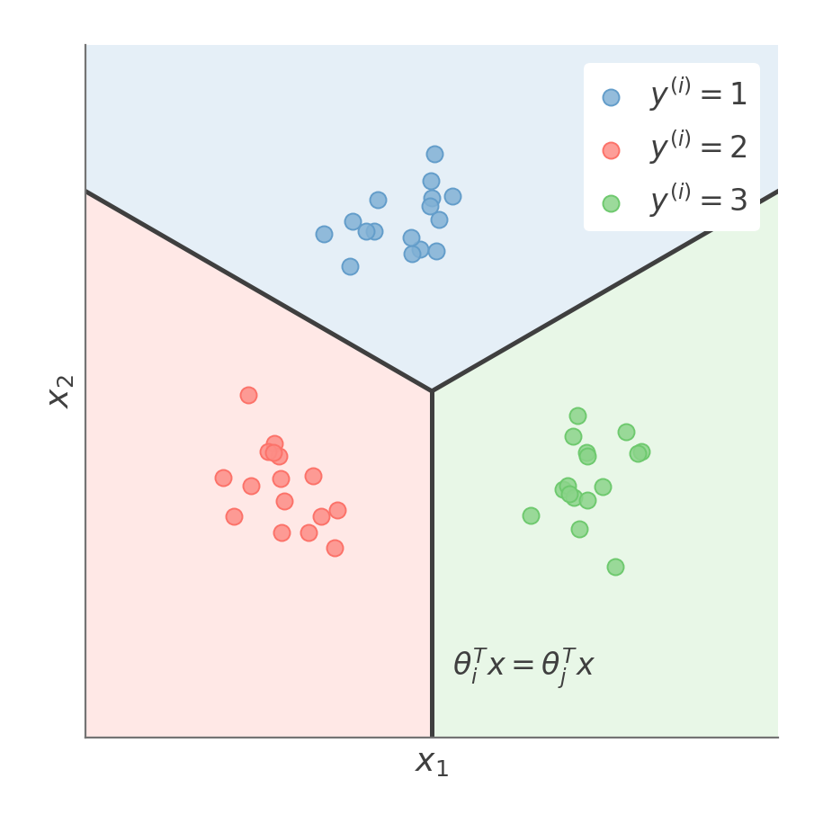
Multiclass Classification

For multi-class classification, if we have $k$ classes, we will have $k * \theta$ parameters and will use a one-vs-all approach.

p(y = i \mid x ; \theta) = \phi_i = \frac{exp\left(\theta_i^T x\right)}{\sum_{j=1}^{k} exp\left(\theta_j^T x\right)}

Softmax decision regions partitioning the feature space into k classes — Softmax assigns each point to the class with the largest score $\theta_i^T x$ , carving the feature space into $k$ regions whose boundaries lie where two classes tie.

Our cross-entropy loss (which is the negative log-likelihood) can then be written as:

\ell_{ce}(\theta) = \sum_{i=1}^m \,- \log \left( \frac{exp\left(\theta_{y^{(i)}}^T x^{(i)}\right)}{\sum_{j=1}^k exp\left(\theta_j^T x^{(i)}\right)} \right)

Taking the derivative of the cross-entropy loss with respect to $\theta_j$ , we get:

\frac{\partial}{\partial \theta_j} \ell_{ce}(\theta) = \sum_{i=1}^m \left( \phi_j^{(i)} - 1\left\{y^{(i)} = j\right\} \right) x^{(i)}

Note that $\phi_j^{(i)} = p(y^{(i)} = j \mid x^{(i)}; \theta)$ .

Therefore, since $\phi_j^{(i)}$ is a probability between 0 and 1, if $y^{(i)} = j$ , we add a negative value of $x^{(i)}$ to our gradient. And if $y^{(i)} \neq j$ , we add a positive value of $x^{(i)}$ to our gradient.

Our gradient descent update rule is then:

\theta_j \leftarrow \theta_j - \alpha \sum_{i=1}^m \left( \phi_j^{(i)} - 1\left\{y^{(i)} = j\right\} \right) x^{(i)}

See derivation

Please use a larger screen

This content is best viewed on a laptop or desktop device.