Expectation Maximization Algorithm

General Formulation

Suppose we have a latent variable model $p(x, z; \theta)$ with $z$ being the latent variable. The density of $x$ can be obtained using marginal probability over $z$ :

p(x; \theta) = \sum_z p(x, z; \theta)

Now to maximize likelihood, we need to maximize the following function:

\ell(\theta) = \sum_{i=1}^n \log p(x^{(i)}; \theta)

= \sum_{i=1}^n \log \sum_{z^{(i)}} p(x^{(i)}; z^{(i)}; \theta)

However, the above equation is not concave with respect to $\theta$ . Hence, we cannot use gradient ascent to find the maximum likelihood estimate.

Moreover, if $p(x; z; \theta)$ is an exponential family distribution, then taking the derivative of the above equation with respect to $\theta$ doesn't typically lead to a solvable expression.

To get around this, we imagine $Q(z)$ to be some distribution over $z$ so that $\sum_z Q(z) = 1$ and $Q(z) \geq 0$

Jensen's Inequality

Jensen's inequality states that for a convex function $[f''(x) \geq 0]$ the following inequality holds:

\mathbb{E}[f(X)] \geq f(\mathbb{E}[X]).

And for concave functions:

\mathbb{E}[f(X)] \leq f(\mathbb{E}[X]).

Also, if $X$ is a constant then $X = \mathbb{E}[X]$ and:

\mathbb{E}[f(X)] = f(\mathbb{E}[X]).

Using Jensen's inequality, we can see that the following inequality holds:

\log p(x; \theta) = \log \sum_z Q(z) \frac{p(x, z; \theta)}{Q(z)}

\geq \sum_z \left[Q(z) \log\frac{p(x, z; \theta)}{Q(z)}\right]

See derivation

From Jensen's inequality, we also know that our inequality becomes an equality (the bound becomes right) when the expectation is over a constant:

\frac{p(x, z; \theta)}{Q(z)} = c

It turns out that this bound is tight when:

Q(z) = p(z | x; \theta)

See derivation

For convenience, let's define Evidence Lower Bound (ELBO) as:

\text{ELBO}(x; Q, \theta) = \mathbb{E}_{z \sim Q(z)}\left[\log\frac{p(x, z; \theta)}{Q(z)}\right] = \sum_z \left[Q(z) \log\frac{p(x, z; \theta)}{Q(z)}\right]

Therefore,

\log p(x; \theta) \geq \text{ELBO}(x; Q, \theta)

\text{Repeat until convergence \{}

\quad \text{(E-step) For each } i, \text{ set } \text{\{}

\quad \quad Q_i(z^{(i)}) \leftarrow p(z^{(i)} | x^{(i)}; \theta)

\quad \text{\}}

\quad \text{(M-step) Set } \text{\{}

\quad \quad \theta \leftarrow \arg \max_{\theta} \sum_{i=1}^{n} \text{ELBO}(x^{(i)}; Q_i, \theta)

\quad \text{\}}

\text{\}}

In the $E$ step we find the estimated distributions over $z^{(i)}$ using our current value of $\theta$ and thus our current estimated distribution over $x^{(i)}$ given $z^{(i)}$ . We do so using the Bayes' rule:

p(z^{(i)} = j | x^{(i)}; \theta) = \frac{p(x^{(i)} | z^{(i)} = j; \theta) p(z^{(i)} = j; \theta)}{\sum_{l=1}^k p(x^{(i)} | z^{(i)} = l; \theta) p(z^{(i)} = l; \theta)}

In the $M$ step we update the value of $\theta$ to maximizes the $\text{ELBO}$ for which it is equal to $\log p(x; \theta)$ for our current values of $\theta$ .

Proof of Convergence

It can be shown that the EM algorithm converges to the maximum likelihood estimate of $\theta$ as the number of iterations goes to infinity.

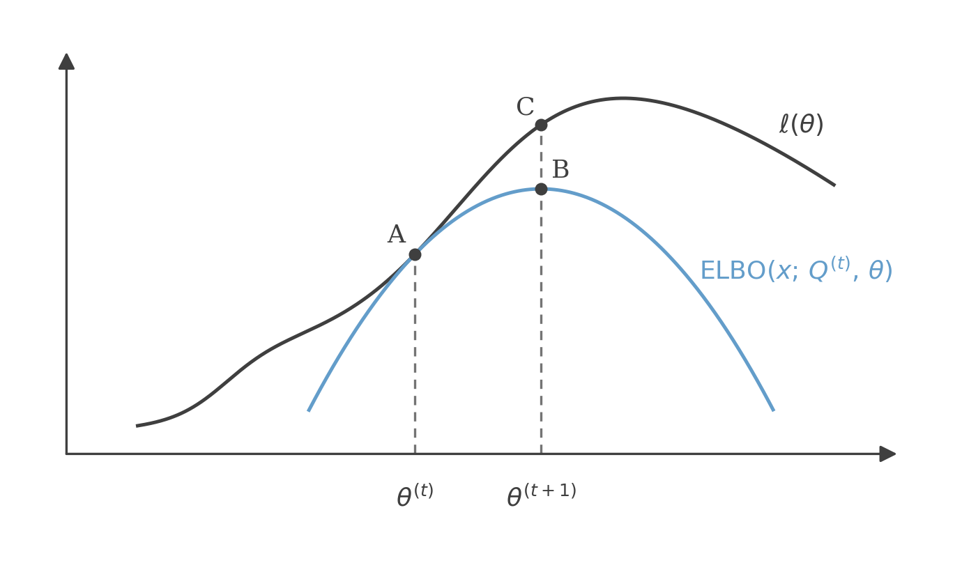
We saw that the for any given value of $\theta$ and any distribution over $z$ , our log-likelihood $\ell(\theta) = \log p(x;\theta)$ is always greater than the $\text{ELBO}(x; Q, \theta)$ .

The ELBO is tangent to the log-likelihood at theta-t; maximizing it reaches theta-(t+1), where the log-likelihood is higher still — For fixed $Q^{(t)}$ , the $\text{ELBO}$ touches $\ell$ at $\theta^{(t)}$ (A); the $M$ -step maximizes it to $\theta^{(t+1)}$ (B), and since $\ell \geq \text{ELBO}$ , $\ell(\theta^{(t+1)})$ (C) is higher still — so a step never decreases $\ell$ .

Hence,

\ell(\theta^{(t+1)}) \geq \sum_{i=1}^{n} \text{ELBO}(x^{(i)}; Q_i^{(t)}, \theta^ {(t+1)})

Moreover, since in the $M$ step, $\theta^{(t+1)}$ is chosen to maximize $\text{ELBO}(x; Q^{(t)}, \theta^ {(t)})$ :

Therefore,

\sum_{i=1}^{n} \text{ELBO}(x^{(i)}; Q_i^{(t)}, \theta^ {(t+1)}) \geq \sum_{i=1}^{n} \text{ELBO}(x^{(i)}; Q_i^{(t)}, \theta^ {(t)})

Finally, in the $E$ step, $Q(z)$ is chosen such that for the current value of $\theta$ , the log-likelihood and the evidence lower bound are equal.

\sum_{i=1}^{n} \text{ELBO}(x^{(i)}; Q_i^{(t)}, \theta^ {(t)}) = \ell(\theta^{(t)})

Putting it all together, we have the following inequality:

\ell(\theta^{(t+1)}) \geq \ell(\theta^{(t)})

Note that the reason we wanted a tight bound on our inequality was to guarantee convergence. Otherwise after the $E$ step, our $\text{ELBO}(x; Q^{(t)}, \theta^{(t)})$ could have been lower than our log-likelihood $\ell(\theta^{(t)})$ . This would've meant that $\ell(\theta^{(t+1)})$ could have been lower than $\ell(\theta^{(t)})$ .

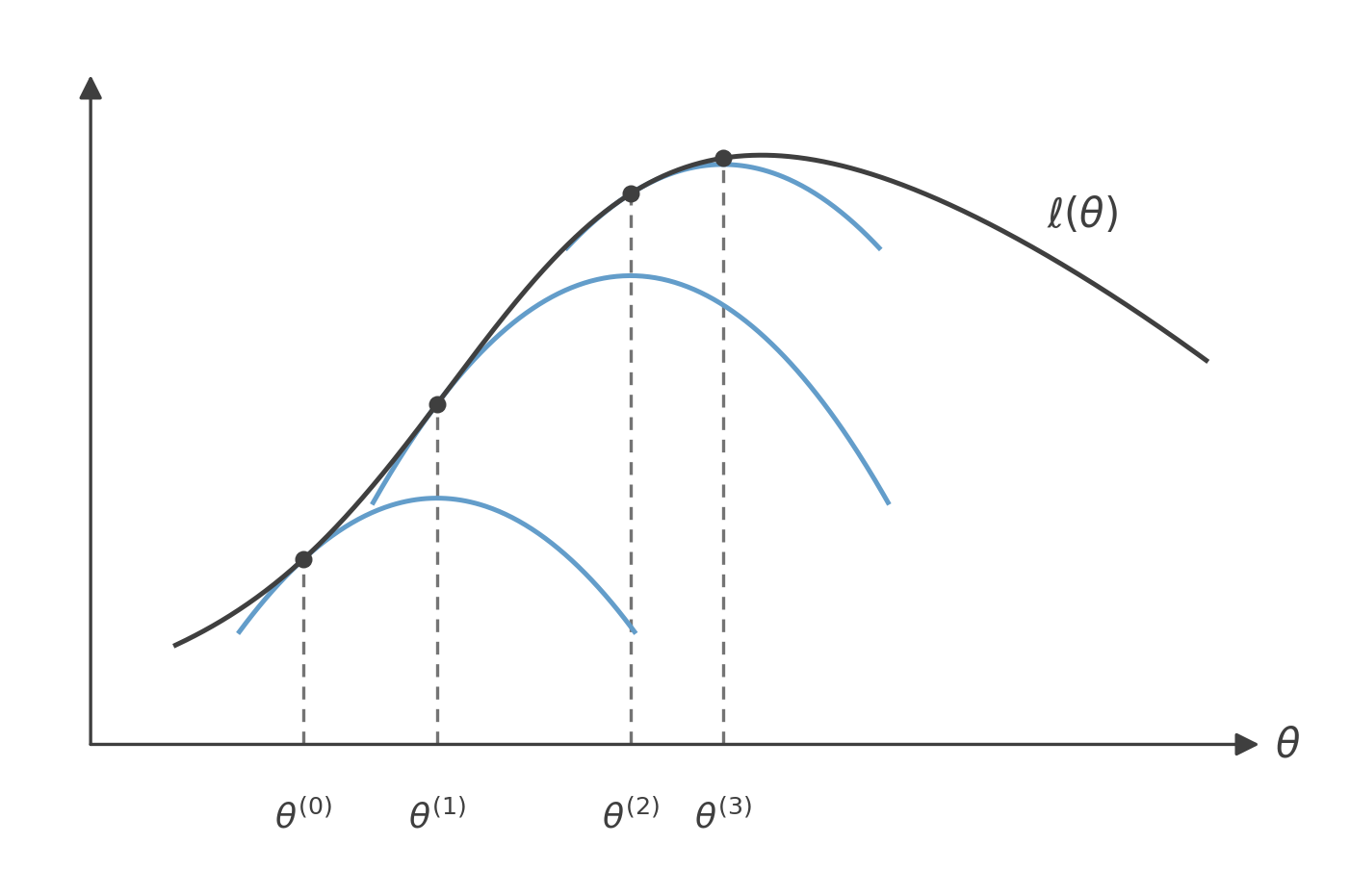
Successive tangent lower bounds climbing the log-likelihood toward a local maximum, with shrinking steps — Repeating the step, each fresh bound is tangent to $\ell$ at the current $\theta^{(k)}$ and is maximized to reach the next iterate; the iterates climb $\ell$ with shrinking steps, converging to a local maximum.

Other Interpretations

The evidence lower bound can be rewritten as:

\text{ELBO}(x; Q, \theta) = \mathbb{E}_{z \sim Q} \left[ \log p(x \mid z; \theta) \right] - D_{KL}(Q \parallel p_z)

This would mean that maximizing $\text{ELBO}$ over $\theta$ is equivalent to maximizing $p(x | z; \theta)$ since the KL-divergence term does not depend on $\theta$ .

See derivation

Similarly, the evidence lower bound can also be rewritten as:

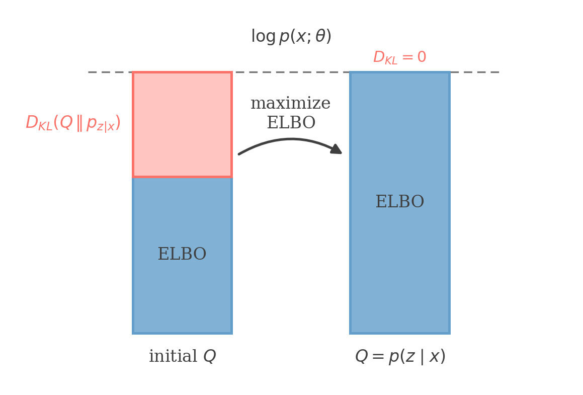
\text{ELBO}(x; Q, \theta) = \log p(x) - D_{KL}(Q \parallel p_{z | x})

This shows us that $\text{ELBO}$ is maximized for a given value of $\theta$ when the KL divergence between $Q(z)$ and $p(z | x; \theta)$ is minimized, which is when they are equal. This is exactly what we saw while deriving the algorithm above.

Log-likelihood split into the ELBO plus the KL gap; setting Q to the posterior closes the gap so the bound is tight — At a fixed $\theta$ , $\log p(x; \theta)$ splits into the $\text{ELBO}$ and the gap $D_{KL}(Q \parallel p_{z | x})$ ; the $E$ step sets $Q = p(z \mid x)$ , closing the gap so the bound is tight.

See derivation

Please use a larger screen

This content is best viewed on a laptop or desktop device.