Generative Learning Algorithms

Gaussian Discriminant Analysis

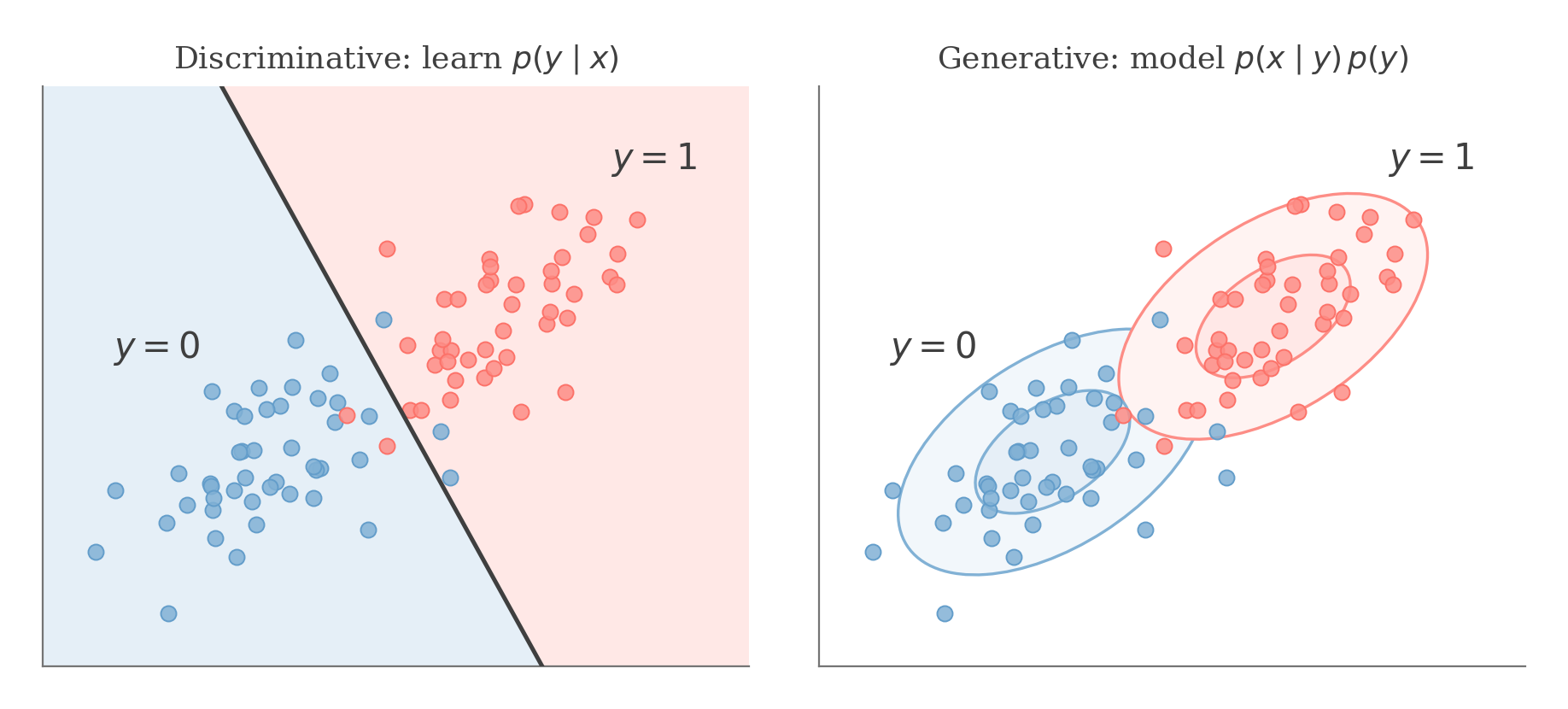
If we want to classify between cats and dogs, discriminative learning algorithms try to learn a hyperplane that separates the two classes directly. Generative learning algorithms, try to learn a model for what cats look like and a separate model to learn what dogs look like.

After modelling $p(x \mid y)$ for each class and the class prior $p(y)$, we can classify a new example by computing the posterior $p(y \mid x)$ for each class and picking the class with the highest posterior probability.

$$\arg \max_y p(y \mid x) = \arg \max_y \, \frac{p(x \mid y) p(y)}{p(x)}$$ $$= \arg \max_y \, p(x \mid y) \, p(y)$$

In Gaussian Discriminant Analysis (GDA), we assume that each of $p(x \mid y)$ follows a multivariate gaussian distribution with unique mean but a shared covariance matrix.

$$p(y) = \phi^y (1 - \phi)^{1 - y}$$ $$p(x \mid y = 0) = \frac{1}{(2 \pi)^{d/2} |\Sigma|^{1/2}} \exp \left( -\frac{1}{2} (x - \mu_0)^T \Sigma^{-1} (x - \mu_0) \right)$$ $$p(x \mid y = 1) = \frac{1}{(2 \pi)^{d/2} |\Sigma|^{1/2}} \exp \left( -\frac{1}{2} (x - \mu_1)^T \Sigma^{-1} (x - \mu_1) \right)$$

The log-likelihood of the data is then given by:

$$\ell(\phi, \mu_0, \mu_1, \Sigma) = \log \prod_{i=1}^n \, p\left(x^{(i)}, y^{(i)}; \phi, \mu_0, \mu_1, \Sigma\right)$$

By maximizing $\ell$ with respect to the parameters, we find the maximum likelihood estimate of the parameters to be:

$$\phi = \frac{1}{n} \sum_{i=1}^n 1\left\{y^{(i)} = 1\right\}$$ $$\mu_0 = \frac{\sum_{i=1}^n 1\left\{y^{(i)} = 0\right\} x^{(i)}}{\sum_{i=1}^n 1\left\{y^{(i)} = 0\right\}}$$ $$\mu_1 = \frac{\sum_{i=1}^n 1\left\{y^{(i)} = 1\right\} x^{(i)}}{\sum_{i=1}^n 1\left\{y^{(i)} = 1\right\}}$$ $$\Sigma = \frac{1}{n} \sum_{i=1}^n \left(x^{(i)} - \mu_{y^{(i)}}\right) \left(x^{(i)} - \mu_{y^{(i)}}\right)^T$$

Naive Bayes

When our feature vectors $x$ take on discrete values, we can use the Naive Bayes.

$$x \in \{0, 1\}^d$$

We also make the assumption that $x_i$'s are conditionally independent given $y$.

$$p(x_1, \ldots, x_d | y) = \prod_{j=1}^d p(x_j | y)$$

We also assume that $y$ takes on two values, $0$ and $1$. Our likelihood function then becomes:

$$\ell(\phi_y, \phi_{j \mid y = 0}, \phi_{j \mid y = 1}) = \log \, \prod_{i=1}^n \, p \left( x^{(i)}, y^{(i)} ; \phi_y, \phi_{j \mid y = 0}, \phi_{j \mid y = 1} \right)$$ $$= \log \, \prod_{i=1}^n \, \left( \prod_{j=1}^d p\left(x_j^{(i)} \mid y^{(i)} ; \phi_{j \mid y = 0}, \phi_{j \mid y = 1}\right) \right) p\left(y^{(i)} ; \phi_y\right)$$

Maximizing our log likelihood function with respect to our parameters, we get:

$$\phi_{j \mid y = 1} = \frac{\sum_{i=1}^{n} 1\left\{x_j^{(i)} = 1 \land y^{(i)} = 1\right\}}{\sum_{i=1}^{n} 1\left\{y^{(i)} = 1\right\}}$$ $$\phi_{j \mid y = 0} = \frac{\sum_{i=1}^{n} 1\left\{x_j^{(i)} = 1 \land y^{(i)} = 0\right\}}{\sum_{i=1}^{n} 1\left\{y^{(i)} = 0\right\}}$$ $$\phi_{y} = \frac{1}{n} \, \sum_{i=1}^{n} 1\left\{y^{(i)} = 1\right\}$$

Having fit all these parameters, to make a prediction on a new example, we simply calculate:

$$p(y = 1|x) = \frac{p(x|y = 1)p(y = 1)}{p(x)}$$ $$p(y = 1|x) = \frac{\left( \prod_{j=1}^{d} p(x_j|y = 1) \right) p(y = 1)}{\left( \prod_{j=1}^{d} p(x_j|y = 1) \right) p(y = 1) + \left( \prod_{j=1}^{d} p(x_j|y = 0) \right) p(y = 0)}$$

However, there is a problem with this approach. If any of the $p(x_j|y = 1)$ is 0, then our prediction will be 0. This happens if we don't have any training example for which a particular $x_j$ is $1$.

As a workaround, we apply Laplace smoothing. Our parameters then become:

$$\phi_{j \mid y = 1} = \frac{1 + \sum_{i=1}^{n} 1\left\{x_j^{(i)} = 1 \land y^{(i)} = 1\right\}}{2 + \sum_{i=1}^{n} 1\left\{y^{(i)} = 1\right\}}$$ $$\phi_{j \mid y = 0} = \frac{1 + \sum_{i=1}^{n} 1\left\{x_j^{(i)} = 1 \land y^{(i)} = 0\right\}}{2 + \sum_{i=1}^{n} 1\left\{y^{(i)} = 0\right\}}$$ $$\phi_y = \frac{1}{n} \, \sum_{i=1}^{n} 1\left\{y^{(i)} = 1\right\}$$