Learning Theory

Bias-Variance Tradeoff

Let $S$ be our set of training examples that are related using the following equation:

y^{(i)} = h^*(x^{(i)}) + \xi^{(i)}

where $h^*$ is the best possible classifier that maps the relationship between $x$ and $y$ , and $\xi^{(i)} \in \mathcal{N}(0, \sigma^2)$ is the noise in the $i$ th example.

Also, let ${h}_s$ be our best fit model for the dataset $S$ . The Mean Squared Error (MSE) can be written as:

\mathbb{E} \left[ (y - h_{s}(x))^2 \right]

Also, let $h_{avg}(x) = \mathbb{E}\left[h_s(x)\right]$ be the "average model" - the model obtained by drawing an infinite number of datasets, training on them, and averaging their predictions on $x$ .

Then, the Mean Squared Error can be further broken down into 3 components:

\mathbb{E} \left[ (y - h_s(x))^2 \right] = \sigma^2 + \underbrace{\left( h^*(x) - h_{\text{avg}}(x) \right)^2}_{\text{bias}^2} + \underbrace{\text{var}(h_s(x))}_{\text{variance}}

The first part is the unavoidable error. It is the noise in the data that cannot be explained by any model, regardless of its complexity.

The bias is the error introduced by the "expressivity handicap" of our classifier. This error occurs because of underfitting.

The variance is the error that measures how much the model's predictions would change if it were trained on a different dataset.

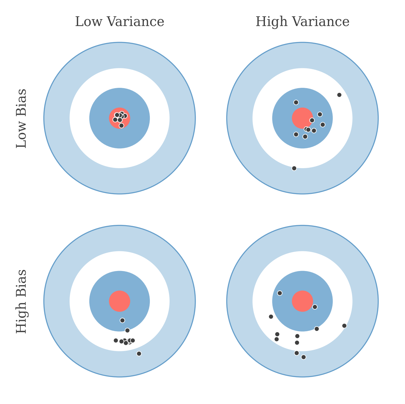
Bias-variance bullseye: four targets showing low and high bias against low and high variance — Each shot is a model fit on a different dataset: bias is how far the cluster sits from the bullseye $h^*$ , while variance is how spread out the shots are.

See derivation

The Bias-Variance tradeoff tells us that as we increase the number of parameters in our neural network, the test error will decrease because the bias is decreasing. However, after a certain point the variance starts increasing faster than the bias is decreasing and therefore, the test error will start to increase.

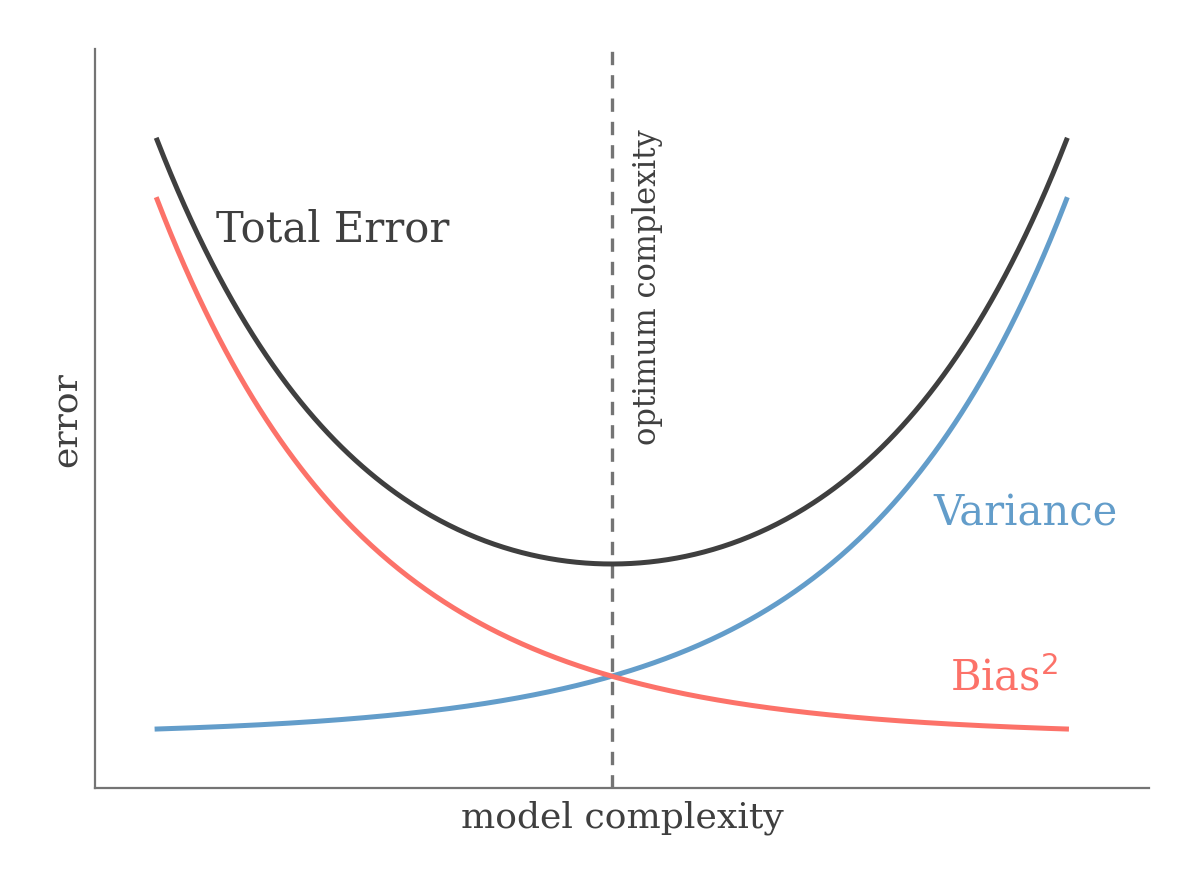
Bias-variance tradeoff: bias squared falling and variance rising, summing to a U-shaped total error — As model complexity grows, $\text{bias}^2$ falls and variance rises; their sum — the total error — is minimized at the intermediate optimum where the two curves cross.

In reality, however, we see a double descent phenomenon wherein the test error starts to decrease again at the point where the number of parameters $d$ are approximately equal to the number of training examples $n$ . This is called the over-parameterization regime.

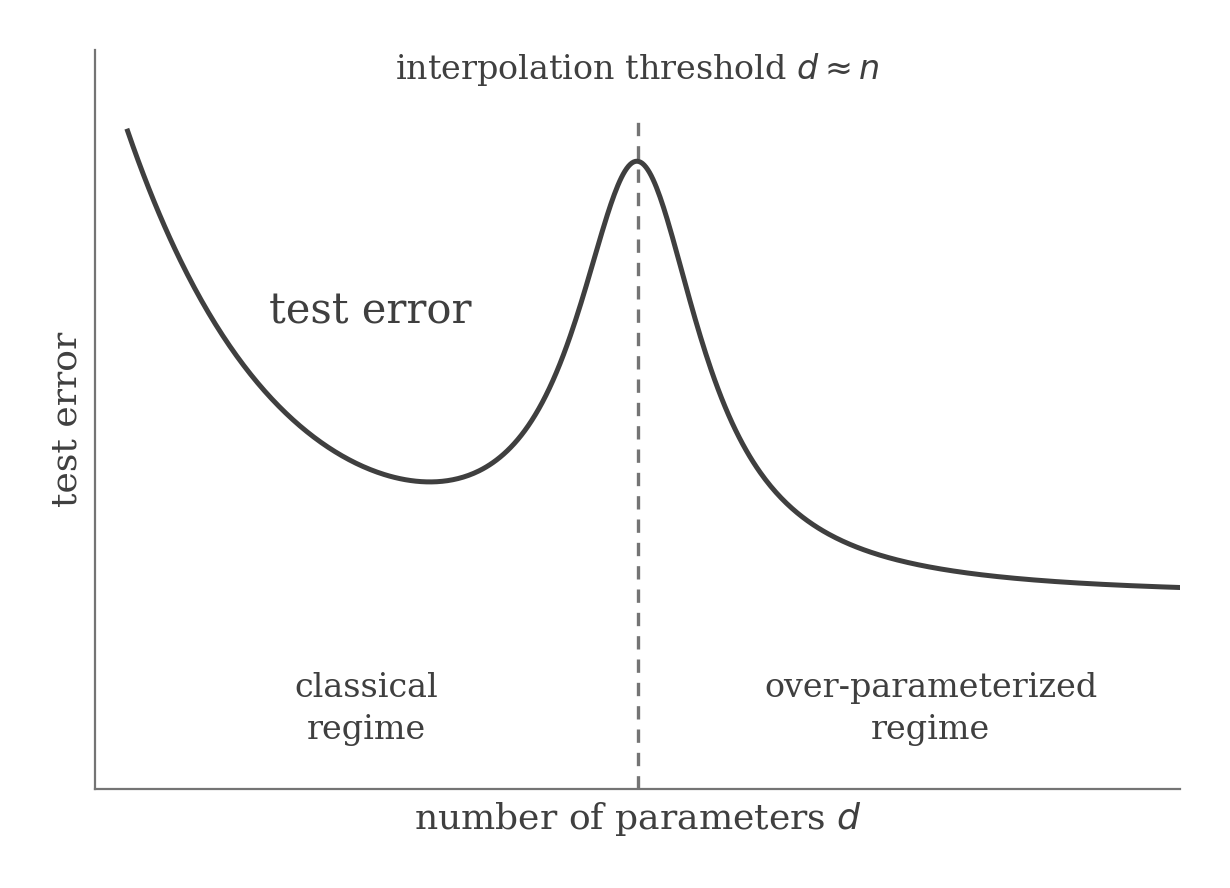
Double descent curve: test error peaks at the interpolation threshold then descends again — Past the interpolation threshold $d \approx n$ , the test error falls a second time, dropping below the classical minimum in the over-parameterized regime.

Complexity Bounds

For any hypothesis $h$ , the true error is given by:

\epsilon(h) = P(h(x) \neq y)

However, since we have no way of determining the underlying probability distribution $\mathcal{D}$ , we cannot determine the true error of the hypothesis. Instead, we estimate the empirical error of the hypothesis over our $n$ training examples.

\hat{\epsilon}(h) = \frac{1}{n} \sum_{i=1}^{n} 1\{h(x_i) \neq y_i\}

Let $\mathcal{H}$ be the set of all possible hypotheses that we are considering. To find the hypothesis that minimizes the empirical error over our training set, we find:

\hat{h} = argmin_{h \in \mathcal{H}} \hat{\epsilon}(h)

Hoeffding Inequality

Hoeffding inequality states that for $n$ independent random variables drawn from a Bernoulli distribution i.e. $P(Z_i = 1) = \phi$ and $P(Z_i = 0) = 1 - \phi$ , the following inequality holds:

P\left( \left|\phi - \hat{\phi}\right| > \gamma \right) \leq 2\exp\left(-2\gamma^2 n\right)

where $\hat{\phi} = \frac{1}{n} \sum_{i=1}^{n} Z_i$ and $\gamma$ is some constant greater than 0.

Imagine a biased coin that comes up heads with a probability of $\phi$ . We toss this coin $n$ times and record the average number of times we got heads. We denote this average by $\hat{\phi}$ .

The probability that "the true probability of getting heads is away from our estimated probability by a difference more than $\gamma$ " is denoted by $P(|\phi - \hat{\phi}| > \gamma)$ . This is always less than or equal to $2\exp\left(-2\gamma^2 n\right)$ .

Using Hoeffding inequality, we note that the true error and the estimated empirical error of our selected hypothesis follow the following inequality:

P\left( \left|\epsilon(h_i) - \hat{\epsilon}(h_i)\right | > \gamma \right) \leq 2\exp\left(-2\gamma^2 n\right)

Now we want to find an inequality for our entire set of hypotheses $\mathcal{H} = \{ h_1, \dots, h_k \}$ . We see that the following inequality holds:

P\left(\forall h \in \mathcal{H}.\left|\epsilon(h_i) - \hat{\epsilon}(h_i)\right | \leq \gamma \right) \geq 1 - 2k\exp\left(-2\gamma^2 n\right)

We call this the uniform convergence result.

This means that as $n$ increases, the probability of the true error being close to the empirical error is bounded by a bigger value. Whereas, as we increase the number of hypotheses in our set, this probability is actually bounded by a smaller value.

In the context of learning, we can say that the more complex our model, the lower our probability of minimizing the empirical error. And the more the number of training examples, the higher our probability of minimizing the empirical error.

See derivation

Now let $\delta = 2k\exp\left(-2\gamma^2 n\right)$

We see that if we want the probability of "the true error being within $\gamma$ to the empirical error for all hypotheses under our consideration" to be at least $1 - \delta$ , our $n$ needs to be at least as large as:

n \geq \frac{1}{2\gamma^2} \log \frac{2k}{\delta}

See derivation

Similarly, we can also see that given $k$ and $n$ , the difference between the true error and the empirical error (for all hypotheses in our set) will always be less than:

\left|\epsilon(h_i) - \hat{\epsilon}(h_i)\right | \leq \sqrt{\frac{1}{2n} \log \frac{2k}{\delta}}

See derivation

Next, in our set of hypotheses $\mathcal{H}$ , let $h^*$ be the hypothesis that minimizes the true error and $\hat{h}$ be the hypothesis that minimizes our empirical error.

Using our uniform convergence assumption, we can see that:

\epsilon(\hat{h}) \leq \epsilon(h^*) + 2\sqrt{\frac{1}{2n} \log \frac{2k}{\delta}}

With a probability of $1 - \delta$ , the true error of our selected hypothesis is less than or equal to the true error of the best hypothesis + some term that depends on the number of hypotheses and the number of training examples.

The first term on the right can be thought of as the bias. And the second term can be thought of as the variance. We see that as we increase k, the first term either stays the same or potentially decreases. Whereas, the second term increases.

This is similar to what we saw in the Bias-Variance tradeoff. As we increase the complexity of our model, variance increases and the potential for our model to overfit also increases.

See derivation

Please use a larger screen

This content is best viewed on a laptop or desktop device.