A Markov Decision Process (MDP) is a mathematical framework used to model decision-making in situations where outcomes are uncertain. It is formulated using a tuple (S,A,Psa,γ,R), where:
S is the set of states.
A is the set of actions.
Psa are the state transition probabilities.
γ is the discount factor.
R is the reward function.
Rewards are usually written as functions of states and actions, i.e. R(s,a) or simply just states, i.e. R(s).
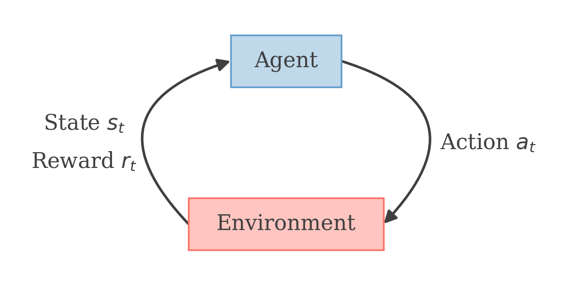
At each step the agent takes an action at, and the environment responds with a new state st+1 and a reward R(st).
Our goal is to find actions that maximize the expected sum of discounted rewards.
E[R(s0)+γR(s1)+γ2R(s2)+...]
A policy is any function π:S→A that maps from states to actions. A value function Vπ is defined as the expected return starting from state s and following policy π.
Vπ(s)=E[R(s0)+γR(s1)+γ2R(s2)+...s0=s,π]
We can write the value function recursively as the Bellman equation:
Note that Psπ(s)(s′) is the probability of landing on state s′ from state s if we take the action π(s).
The optimal value function V∗(s) is the maximum value function over all policies:
V∗(s)=πmaxVπ(s)
The Bellman equation for the optimal value function is:
V∗(s)=R(s)+a∈Amax(γs′∈S∑Psa(s′)V∗(s′))
The optimal policy π∗ is the one that maximizes the value function:
π∗(s)=arga∈Amax(s′∈S∑Psa(s′)V∗(s′))
Finding the optimal policy is equivalent to finding the optimal value function. And there are two algorithms that can do this: Value Iteration and Policy Iteration.
Value IterationFor each state s, initialize V(s)=0Repeat until convergence {For each state s, set {V(s)←R(s)+a∈Amax(γs′∈S∑Psa(s′)V(s′))}}
Policy IterationInitialize π randomlyRepeat until convergence {Let V=Vπ⇒typically by a linear system solverFor each state s, set {π(s)←arga∈Amax(s′∈S∑Psa(s′)V(s′))}}
For small MDPs, Policy iteration converges faster. However, for large MDPs, solving for Vπ in each step of policy iteration involves solving a large system of linear equations, which is computationally expensive.
Usually, we do not know the state transition probabilities Psa beforehand. Instead, they can be estimated by repeatedly running the agent on the MDP under policy π and using the following formula:
Psa(s′)=# of times we took action a in state s# of times we took action a in state s and ended up in state s′
Value Function Approximation
One way to deal with continuous state spaces in MDPs is to discretize the state space. If we have d dimensions and we discretize each dimension with k values, then we have kd states. As we increase k, the number of states grows exponentially.
To deal with this, we can use function approximation.
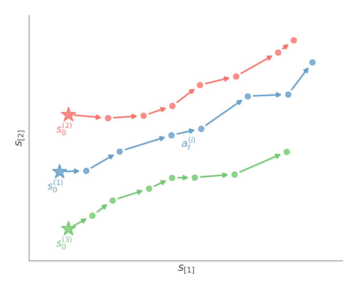
One way to do this is using a model-based approach. We use a simulator to execute n trials, each for T time steps.
However, this is a deterministic model. Most real world systems are stochastic. So we can modify the model to be stochastic by adding a noise term:
st+1=Ast+Bat+ϵϵ∼N(0,Σ)
Now, if we assume that our state space is continuous but our action space is small and discrete, we can use the Fitted value iteration algorithm.
st+1−(Ast+Bat)=ϵ
Since ϵ is normally distributed, the term st+1−(Ast+Bat) is also normally distributed. We can then write:
st+1∼N(Ast+Bat,Σ)
Our state transition function can now be written as:
Psa(s′)=N(As+Ba,Σ)
Moreover, our value iteration update rule for the continuous case can be written as:
V(s)←R(s)+γ⋅a∈Amax(∫s′Psa(s′)V(s′)ds′)
However, since our states s are continuous, we have to approximate the value function V(s) as well. We do so by finding a linear or non-linear mapping from states to the value function:
V(s)=θTϕ(s)
We also cannot directly update our V(s) from the value iteration update rule. Instead, we have to update our θ parameters.
Randomly sample n statesInitialize θ to 0Repeat until convergence {For i=1 to n {For each action a∈A {Sample s1′,s2′,…,sk′∼Ps(i)a(s′)Set q(a)←R(s(i))+γ⋅k1⋅j=1∑kV(sj′)}y(i)←amaxq(a)}θ←argθmini=1∑n(y(i)−θTϕ(s(i)))2}
Please use a larger screen
This content is best viewed on a laptop or desktop device.