Decision Trees

Introduction

In the K-means Algorithm, we made an inherent assumption that data points of various classes are not randomly sprinkled across the space, but instead appear in cluseters of more or less homogeneous space.

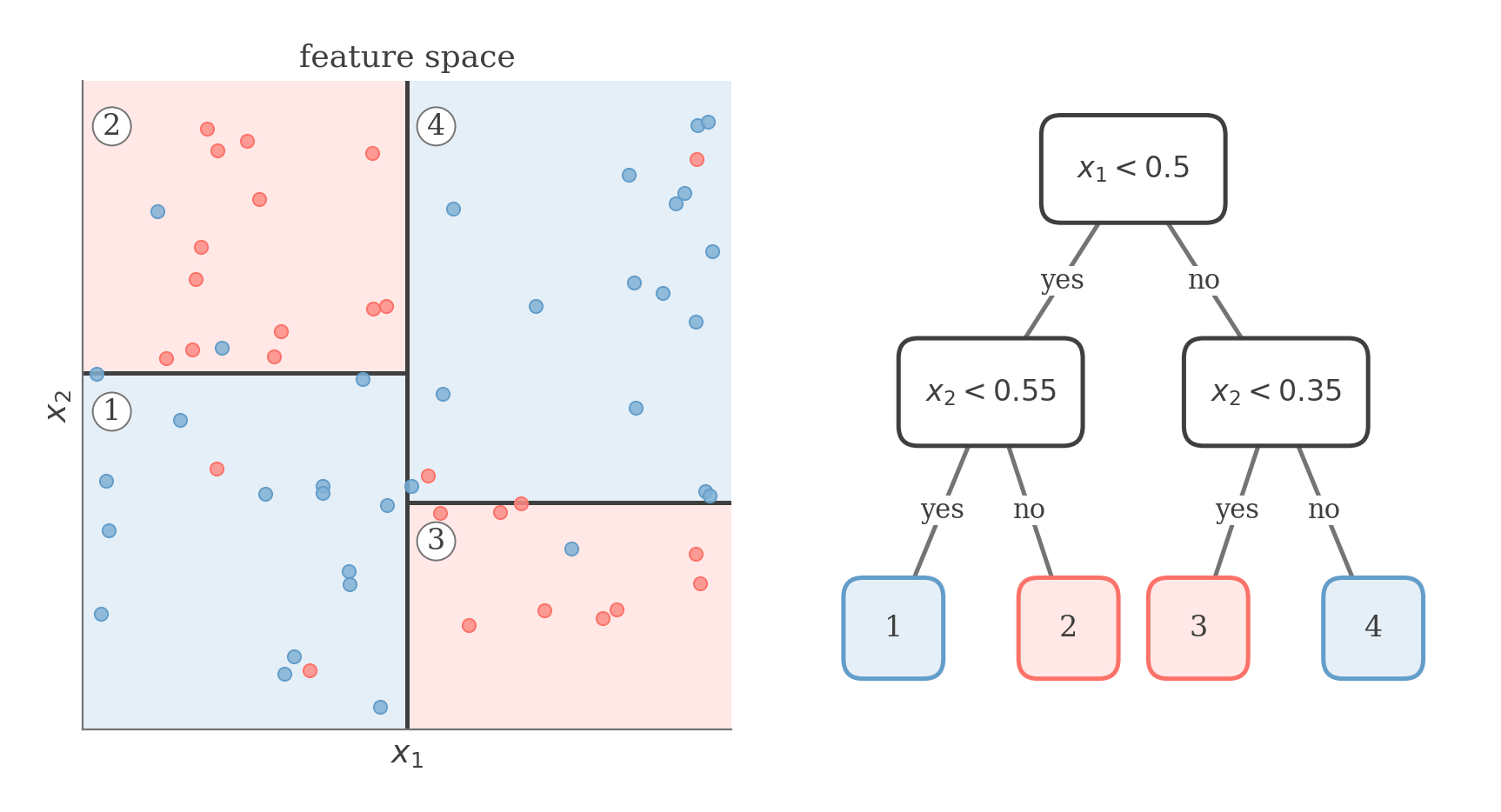
Decision trees exploit this very assumption to build a tree structure that recursively divides the feature space into regions with similar labels.

For this purpose, we use the concept of purity. We want to split the data at each node such that the resulting subsets are as pure as possible.

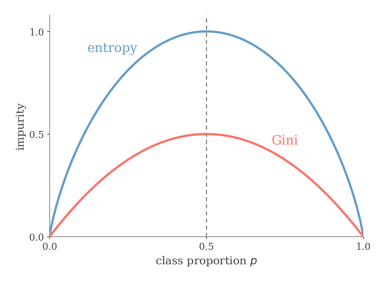
Two common impurity measures are Gini impurity and entropy.

Let $S = \{(x^{(1)}, y^{(1)}), \ldots, (x^{(n)}, y^{(n)})\}$ be a set of training examples where $y^{(i)} \in \{1, \ldots, c\}$ for $c$ classes. Then we can define the probability of any class $k$ as:

$$p_k = \frac{|S_k|}{|S|}$$

The Gini impurity of a leaf $S$ is given by:

$$G(S) = \sum_{k=1}^c p_k (1 - p_k)$$

And for a split $S \rightarrow S_L, \, S_R$, the Gini impurity is given by:

$$G(S) = \frac{|S_L|}{|S|} \cdot G(S_L) + \frac{|S_R|}{|S|} \cdot G(S_R)$$

Similarly, the entropy of a leaf $S$ is given by:

$$H(S) = - \sum_{k=1}^c p_k \log p_k$$

And for a split $S \rightarrow S_L, \, S_R$, the entropy impurity is given by:

$$H(S) = \frac{|S_L|}{|S|} \cdot H(S_L) + \frac{|S_R|}{|S|} \cdot H(S_R)$$

Also, note that the worst case for our probabilities is if they follow a uniform distribution and $p_k = \frac{1}{c}$ for each $k$ because this would mean that each leaf is equally likely and our predictions are as good as random guessing.

If we let this distribution be $q$ then we see that minimizing the entropy is equivalent to maximizing the KL-divergence $D_{KL}(p || q)$.

$$\arg \max_p D_{KL}\left(p \, || \, q\right) = \arg \min_p \left( - \sum_k p_k \, \log p_k \right)$$ $$= \arg \min_p H(p)$$

However, building a maximally compact tree with only pure leaves for any data set is a NP-hard problem. Therefore, we use a greedy approach instead.

One example of this is the ID3 algorithm. In this algorithm, we start at the root node and at each step select the feature $x_j$ that best separates the data and minimizes the impurity. We then recurse on the left and right subsets defined by this split until we can no longer split the data.

A problem with this approach is that the ID3 algorithm stops splitting if a single split doesn't reduce impurity, even though a combination of splits might.

Another example of the greedy approach is the CART (Classification and Regression Trees) algorithm. CART can handle both classification and regression tasks. For regression tasks, the cost function is the squared error and for classification tasks it is the Gini impurity or entropy.

Bagging

From Bias-Variance Tradeoff, we know that the Mean Squared Error (MSE) between the best possible classifier and our classifier can be broken down.

$$\mathbb{E} \left[ (y - h_s(x))^2 \right] = \sigma^2 + \underbrace{\left( h^*(x) - h_{\text{avg}}(x) \right)^2}_{\text{bias}^2} + \underbrace{\mathbb{E}\left[\left(h_{avg}(x) - h_{s}(x)\right)^2 \right]}_{\text{variance}}$$

The variance term indicates how much the model's predictions would change if it were trained on a different dataset.

If we let $D_i$ be the $i$th dataset, then for $n$ datasets, we can define the average model as the ensemble average:

$$\hat{h}(x) = \frac{1}{n} \sum_{j=1}^{n} h_{D_i}(x)$$

As $n \to \infty$, according to the Law of Large Numbers, our average model $\hat{h}(x)$ will converge to $h_{avg}(x)$.

This means that if we have infinite datasets and we train our classifiers on each data set and then take an average, we can reduce the variance to $0$.

However, we do not have infinite datasets, we only have one. Therefore, we use Bootstraping instead. We sample $n$ datasets with replacement from our original dataset $D$.

Note that doing this means that our datasets are not independent and identically distributed and according to the Law of Large Numbers is no longer guaranteed. In practice, however, doing this still helps us reduce the variance to some extent.

Next, to find the unbiased estimate of the test error, we need to find the out-of-bag (OOB) error.

Let $S_i$ be the set of all sampled data sets that do not contain the $i$th example. Then our prediction for the $i$th example is given by:

$$\tilde{h}_i(x) = \frac{1}{|S_i|} \sum_{j \in S_i} h_{j}(x)$$

Then the out-of-bag error is given by:

$$\epsilon_{\text{oob}} = \frac{1}{n} \sum_{i=1}^{|D|} \, loss\left(\tilde{h}_i(x^{(i)}), \, y^{(i)}\right)$$

Random Forest is an example of Bagging. In Random Forest, each decision tree is trained on a bootstrapped sample of the data, and only a random subset of $k$ features are considered for splitting at each node. Each tree is grown to its full depth, and then an ensemble average is used to make predictions.

Usually $k = \sqrt{d}$ where $d$ is the total number of features in each example.

Boosting

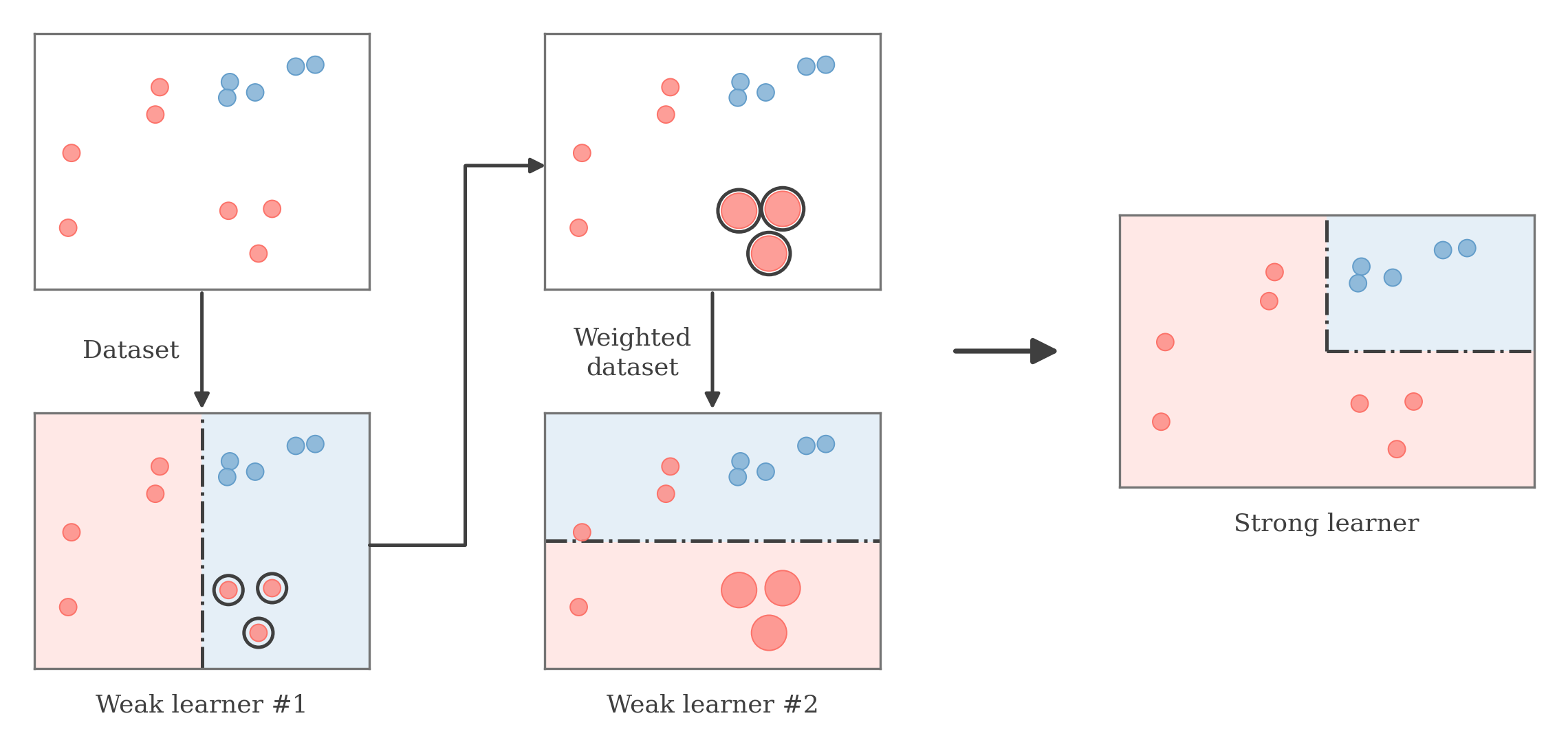
Boosting uses an ensemble of weak learners, added in an iterative manner, to form a strong learner with low bias.

In each iteration, we find a classifier $h$ from our set of classifiers $\mathcal{H}$ that minimizes the loss function $\ell$.

$$h_{t+1} = \arg \min_{h \in \mathcal{H}} \, \ell(H_t + \alpha h)$$

Our ensemble classifier can thus be written as:

$$H_{t}(x) = \sum_{i=1}^{t} \alpha_i h_i(x)$$

To find the classifier that minimizes the loss function at any given step, we can use gradient descent in function space.

$$h_{t+1} = \arg \min_{h \in \mathcal{H}} \, \ell(H_t + \alpha h)$$

This can be rewritten as:

$$h_{t+1} = \arg \min_{h \in \mathcal{H}} \, \left[ \sum_{i=1}^{n} \frac{\partial \ell}{\partial H_t\left(x^{(i)}\right)} \cdot h\left(x^{(i)}\right) \right]$$

If $\ell$ is the square loss function, we can further rewrite this as:

$$h_{t+1} = \arg \min_{h \in \mathcal{H}} \, \left[ \sum_{i=1}^{n} \left(H_t(x^{(i)}) - y^{(i)}\right) \cdot h(x^{(i)}) \right]$$

Note that $y^{(i)} - H_t\left(x^{(i)}\right)$ represents the vector from $H_t\left(x^{(i)}\right)$ to $y^{(i)}$. Therefore, any $h_{t+1}$ that moves us closer to $y^{(i)}$ will have a high dot product with this vector.

From this it follows that such a vector will have a negative dot product with $H_t\left(x^{(i)}\right) - y^{(i)}$.

Therefore, we want to select $h_{t+1}$ such that:

$$\left[H_t\left(x^{(i)}\right) - y^{(i)}\right] \cdot h_{t+1}\left(x^{(i)}\right) \lt 0$$

We can use this observation to write a Generic Boosting algorithm.

def create_updated_ensemble(current_H, alpha, new_h):
    """Create new ensemble: H_new = H_old + alpha * h"""
    return lambda x: current_H(x) + alpha * new_h(x)

# Initialize ensemble classifier
H = lambda x: 0  # Start with zero function
    
for iteration in range(max_iterations):
    # Compute gradients for each training example
    gradients = []
    for i in range(len(X)):
        r_i = compute_gradient(loss_function, H(X[i]), y[i])
        gradients.append(r_i)
        
    # Find the best weak learner that minimizes the gradient dot product
    best_h = None
    min_score = float('inf')
        
    for h in H_set:
        score = 0
        for i in range(len(X)):
            score += gradients[i] * h(X[i])
        
        if score < min_score:
            min_score = score
            best_h = h
        
    if min_score < 0:
        # Update ensemble classifier
        H = create_updated_ensemble(H, alpha, best_h)
    else:
        # No improvement possible, stop boosting
        break

AdaBoost

AdaBoost is a boosting algorithm that is used for classification tasks.

We assume that $y^{(i)} \in \{-1, 1\}$ and $h(x) \in \{-1, 1\}$.

We also use an exponential loss function:

$$\ell(H) = e^{-y^{(i)} \cdot H(x^{(i)})}$$

The gradient of this loss function is given by:

$$\frac{\partial \ell}{\partial H(x^{(i)})} = -y^{(i)} \cdot e^{-y^{(i)} \cdot H(x^{(i)})}$$

Using this gradient, we can see that the best classifier $h_t$ is the one that minimizes the loss function can be written as a weighted misclassification error:

$$h_{t+1} = \arg \min_{h \in \mathcal{H}} \left( \sum_{i=1}^{n} \mathbb{1}\left\{y^{(i)} \neq h(x^{(i)})\right\} \cdot w^{(i)} \right)$$ $$w^{(i)} = \frac{\exp\left(-y^{(i)} \cdot H_t(x^{(i)})\right)}{\sum_{j=1}^{n} \exp\left(-y^{(j)} \cdot H_t(x^{(j)})\right)}$$

We can further divide our weights $w^{(i)}$ in terms of unnormalized weights $\hat{w}^{(i)}$ and a normalization constant $z$.

$$w^{(i)} = \frac{1}{z} \cdot \hat{w}^{(i)}$$ $$\hat{w}^{(i)} = e^{-y^{(i)} \cdot H_t(x^{(i)})}$$ $$z = \sum_{j=1}^{n} e^{-y^{(j)} \cdot H_t(x^{(j)})}$$

In AdaBoost, we can also find the optimal step size by minimizing the loss function with respect to $\alpha$.

$$\alpha = \arg \min_{\alpha} \ell(H_t + \alpha h)$$

Doing so, we find a closed form solution for the optimal step size in terms of the weighted classification error.

$$\alpha = \frac{1}{2} \ln\left(\frac{1 - \epsilon}{\epsilon}\right)$$ $$\epsilon = \sum_{i=1}^{n} 1\left\{y^{(i)} \neq h(x^{(i)})\right\} \cdot w^{(i)}$$

After taking each step, we need to recompute our weights and renormalize them so that they sum to one.

The update rules for the unnormalized weights and normalization constant are given by:

$$\hat{w}^{(i)} \leftarrow \hat{w}^{(i)} \cdot e^{-\alpha y^{(i)} h(x^{(i)})}$$ $$z \leftarrow z * 2 \sqrt{\epsilon(1 - \epsilon)}$$

Putting these together, we get the following update rule for the normalized weights:

$$w^{(i)} \leftarrow w^{(i)} \cdot \frac{e^{-\alpha y^{(i)} h(x^{(i)})}}{2 \sqrt{\epsilon(1 - \epsilon)}}$$

Note that when $\epsilon = \frac{1}{2}$, that means that our weighted misclassification error is equal to $50\%$. This means that our new classifier $h_{t+1}$ is no better than random guessing. Therefore, we only want to add a new classifier to our current ensemble if $\epsilon < \frac{1}{2}$.

def create_updated_ensemble(current_H, alpha, new_h):
    """Create new ensemble: H_new = H_old + alpha * h"""
    return lambda x: current_H(x) + alpha * new_h(x)

n = len(X)

# Initialize weights uniformly
weights = np.ones(n) / n

# Initialize ensemble classifier
H = lambda x: 0  # Start with zero function

for iteration in range(max_iterations):
    # Find best weak learner that minimizes weighted classification error
    best_h = None
    min_error = float('inf')
    
    for h in H_set:
        # Compute weighted misclassification error
        error = 0
        for i in range(n):
            if y[i] != h(X[i]):  # Misclassification indicator
                error += weights[i]
        
        if error < min_error:
            min_error = error
            best_h = h
    
    epsilon = min_error
    
    # Check stopping condition
    if epsilon >= 0.5:
        # Weak learner is no better than random guessing
        break
    
    # Compute step size (alpha)
    alpha = 0.5 * math.log((1 - epsilon) / epsilon)
    
    # Update ensemble using the helper function
    H = create_updated_ensemble(H, alpha, best_h)
    
    # Update weights
    normalization_factor = 2 * math.sqrt(epsilon * (1 - epsilon))
    
    for i in range(n):
        # Update weight based on classification result
        prediction = best_h(X[i])
        weights[i] = weights[i] * math.exp(-alpha * y[i] * prediction) / normalization_factor