Linear Regression
Linear regression predicts a continuous value using a linear function of the input features.
Given an input x x x θ \theta θ y y y
To include an intercept, we set x 0 ( i ) = 1 x_0^{(i)}=1 x 0 ( i ) = 1 x ( i ) ∈ R d + 1 x^{(i)}\in\mathbb{R}^{d+1} x ( i ) ∈ R d + 1 d d d θ ∈ R d + 1 \theta\in\mathbb{R}^{d+1} θ ∈ R d + 1
The model predicts:
h θ ( x ) = ∑ j = 0 d θ j x j = θ T x
h_{\theta}(x)
=
\sum_{j=0}^{d}
\theta_jx_j
=
\theta^Tx
h θ ( x ) = j = 0 ∑ d θ j x j = θ T x For training example i i i
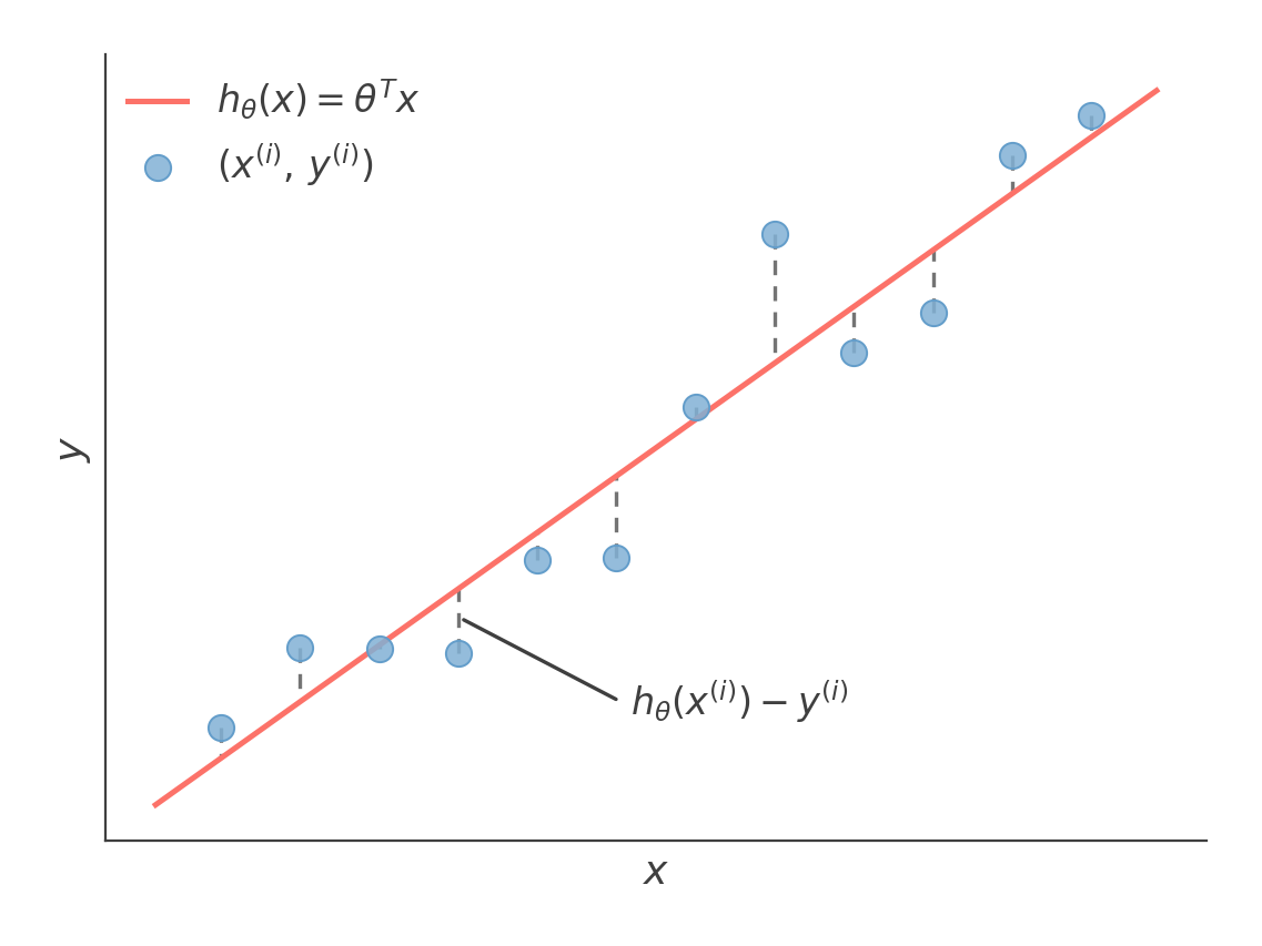
h θ ( x ( i ) ) − y ( i )
h_\theta(x^{(i)})-y^{(i)}
h θ ( x ( i ) ) − y ( i ) is called the residual.
We measure the total error by adding the squared residuals across the training set:
J ( θ ) = 1 2 ∑ i = 1 n ( h θ ( x ( i ) ) − y ( i ) ) 2
J(\theta)
=
\frac12
\sum_{i=1}^{n}
\left(
h_{\theta}(x^{(i)})
-
y^{(i)}
\right)^2
J ( θ ) = 2 1 i = 1 ∑ n ( h θ ( x ( i ) ) − y ( i ) ) 2 Our goal is to choose θ \theta θ J ( θ ) J(\theta) J ( θ )
The cost function measures the squared vertical residuals between each training label and the fitted line.
To minimize J ( θ ) J(\theta) J ( θ ) θ j \theta_j θ j
Taking the derivative gives:
∂ ∂ θ j J ( θ ) = ∑ i = 1 n [ h θ ( x ( i ) ) − y ( i ) ] x j ( i ) , j = 0 , … , d
\frac{\partial}{\partial\theta_j}
J(\theta)
=
\sum_{i=1}^{n}
\left[
h_\theta(x^{(i)})
-
y^{(i)}
\right]
x_j^{(i)},
\qquad
j=0,\ldots,d
∂ θ j ∂ J ( θ ) = i = 1 ∑ n [ h θ ( x ( i ) ) − y ( i ) ] x j ( i ) , j = 0 , … , d This derivative tells us how changing θ j \theta_j θ j
› See derivation∂ ∂ θ j J ( θ ) = ∂ ∂ θ j [ 1 2 ∑ i = 1 n ( h θ ( x ( i ) ) − y ( i ) ) 2 ]
\frac{\partial}{\partial \theta_j} J(\theta)
=
\frac{\partial}{\partial \theta_j}
\left[
\frac{1}{2}
\sum_{i=1}^{n}
\left(
h_{\theta}(x^{(i)}) - y^{(i)}
\right)^2
\right]
∂ θ j ∂ J ( θ ) = ∂ θ j ∂ [ 2 1 i = 1 ∑ n ( h θ ( x ( i ) ) − y ( i ) ) 2 ] = ∑ i = 1 n [ 2 ⋅ 1 2 ( h θ ( x ( i ) ) − y ( i ) ) ⋅ ∂ ∂ θ j ( h θ ( x ( i ) ) − y ( i ) ) ]
=
\sum_{i=1}^{n}
\left[
2\cdot\frac12
\left(
h_\theta(x^{(i)})-y^{(i)}
\right)
\cdot
\frac{\partial}{\partial\theta_j}
\left(
h_\theta(x^{(i)})-y^{(i)}
\right)
\right]
= i = 1 ∑ n [ 2 ⋅ 2 1 ( h θ ( x ( i ) ) − y ( i ) ) ⋅ ∂ θ j ∂ ( h θ ( x ( i ) ) − y ( i ) ) ] = ∑ i = 1 n [ ( h θ ( x ( i ) ) − y ( i ) ) ⋅ ∂ ∂ θ j ( ∑ k = 0 d θ k x k ( i ) − y ( i ) ) ]
=
\sum_{i=1}^{n}
\left[
\left(
h_\theta(x^{(i)})-y^{(i)}
\right)
\cdot
\frac{\partial}{\partial\theta_j}
\left(
\sum_{k=0}^{d}\theta_kx_k^{(i)}
-
y^{(i)}
\right)
\right]
= i = 1 ∑ n [ ( h θ ( x ( i ) ) − y ( i ) ) ⋅ ∂ θ j ∂ ( k = 0 ∑ d θ k x k ( i ) − y ( i ) ) ] = ∑ i = 1 n [ ( h θ ( x ( i ) ) − y ( i ) ) ⋅ ∂ ∂ θ j ( θ j x j ( i ) ) ]
=
\sum_{i=1}^{n}
\left[
\left(
h_\theta(x^{(i)})-y^{(i)}
\right)
\cdot
\frac{\partial}{\partial\theta_j}
\left(
\theta_jx_j^{(i)}
\right)
\right]
= i = 1 ∑ n [ ( h θ ( x ( i ) ) − y ( i ) ) ⋅ ∂ θ j ∂ ( θ j x j ( i ) ) ] i The other terms do not depend on θ j \theta_j θ j
= ∑ i = 1 n [ ( h θ ( x ( i ) ) − y ( i ) ) x j ( i ) ]
=
\sum_{i=1}^{n}
\left[
\left(
h_\theta(x^{(i)})-y^{(i)}
\right)
x_j^{(i)}
\right]
= i = 1 ∑ n [ ( h θ ( x ( i ) ) − y ( i ) ) x j ( i ) ] Instead of computing the gradient over the entire dataset before every update, stochastic gradient descent uses one training example at a time.
For training example i i i
θ ← θ + α ( y ( i ) − h θ ( x ( i ) ) ) x ( i )
\theta
\leftarrow
\theta
+
\alpha
\left(
y^{(i)}
-
h_\theta(x^{(i)})
\right)
x^{(i)}
θ ← θ + α ( y ( i ) − h θ ( x ( i ) ) ) x ( i ) where α > 0 \alpha>0 α > 0
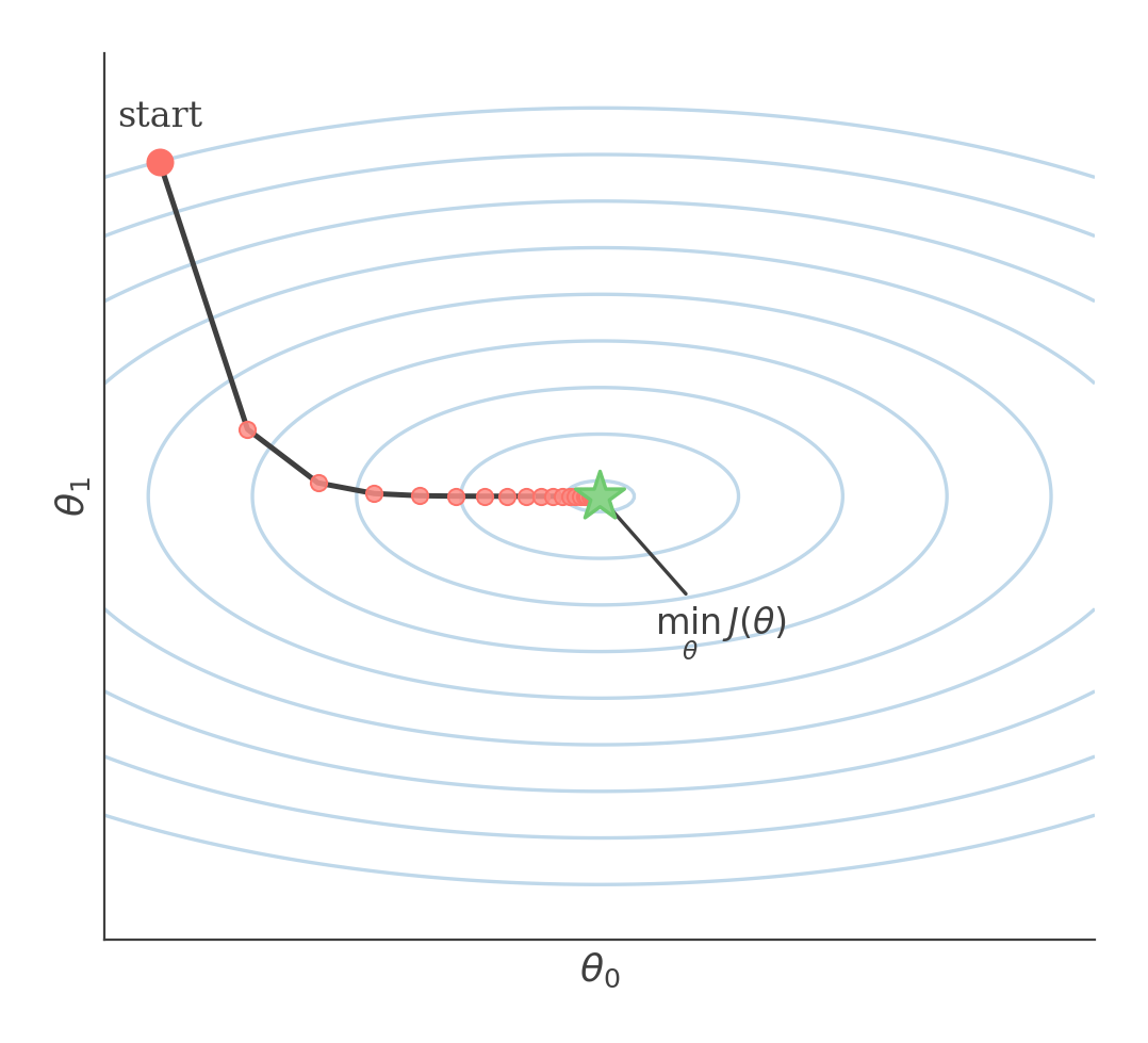
Gradient descent updates θ \theta θ J ( θ ) J(\theta) J ( θ )
Repeat until convergence {
\text{Repeat until convergence \{}
Repeat until convergence { For i = 1 to n , {
\quad
\text{For } i=1 \text{ to } n,\text{ \{}
For i = 1 to n , { θ ← θ + α ( y ( i ) − h θ ( x ( i ) ) ) x ( i )
\quad\quad
\theta
\leftarrow
\theta
+
\alpha
\left(
y^{(i)}
-
h_\theta(x^{(i)})
\right)
x^{(i)}
θ ← θ + α ( y ( i ) − h θ ( x ( i ) ) ) x ( i ) }
\quad
\text{\}}
} }
\text{\}}
} Gradient descent finds the parameters through repeated updates. For ordinary least squares, we can also solve for the optimal parameters directly.
Let X ∈ R n × ( d + 1 ) X\in\mathbb{R}^{n\times(d+1)} X ∈ R n × ( d + 1 )
y ⃗ = [ y ( 1 ) ⋮ y ( n ) ]
\vec y
=
\begin{bmatrix}
y^{(1)}\\
\vdots\\
y^{(n)}
\end{bmatrix}
y = y ( 1 ) ⋮ y ( n ) The predictions for the entire dataset can then be written as:
y ⃗ ^ = X θ
\hat{\vec y}
=
X\theta
y ^ = Xθ Using the fact that z T z = ∑ i z i 2 z^Tz=\sum_i z_i^2 z T z = ∑ i z i 2
J ( θ ) = 1 2 ∑ i = 1 n ( h θ ( x ( i ) ) − y ( i ) ) 2
J(\theta)
=
\frac12
\sum_{i=1}^{n}
\left(
h_{\theta}(x^{(i)})
-
y^{(i)}
\right)^2
J ( θ ) = 2 1 i = 1 ∑ n ( h θ ( x ( i ) ) − y ( i ) ) 2 = 1 2 ( X θ − y ⃗ ) T ( X θ − y ⃗ )
=
\frac12
\left(
X\theta-\vec y
\right)^T
\left(
X\theta-\vec y
\right)
= 2 1 ( Xθ − y ) T ( Xθ − y ) Setting the gradient to zero gives the normal equations:
X T X θ = X T y ⃗
X^TX\theta
=
X^T\vec y
X T Xθ = X T y If X X X
θ ⋆ = ( X T X ) − 1 X T y ⃗
\theta^\star
=
\left(
X^TX
\right)^{-1}
X^T\vec y
θ ⋆ = ( X T X ) − 1 X T y If X T X X^TX X T X
θ ⋆ = X + y ⃗
\theta^\star
=
X^+\vec y
θ ⋆ = X + y where X + X^+ X +
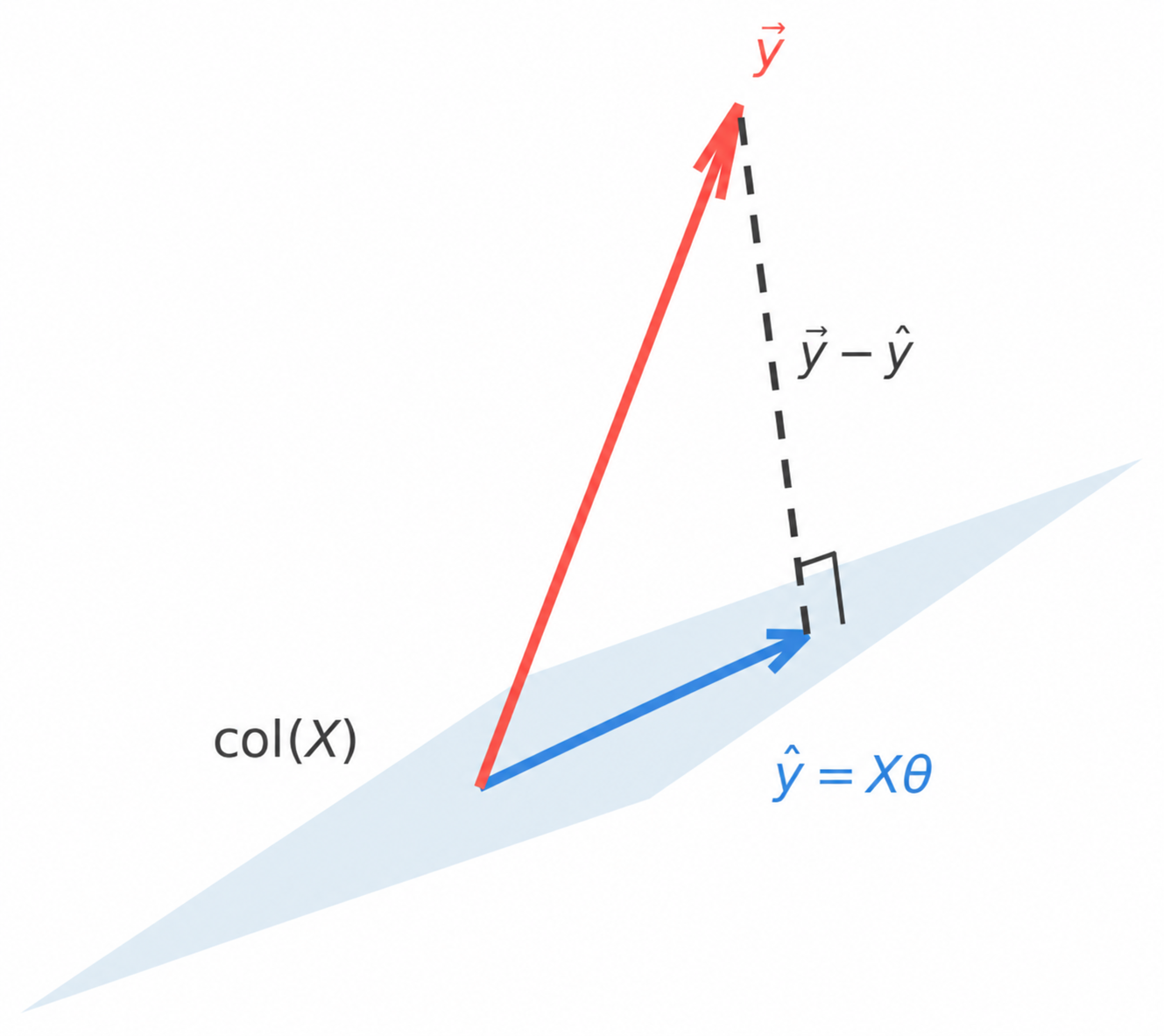
The closed-form solution chooses the prediction vector y ^ = X θ \hat{y} = X\theta y ^ = Xθ y ⃗ \vec{y} y X X X
› See derivation∇ θ J ( θ ) = ∇ θ ( 1 2 ( X θ − y ⃗ ) T ( X θ − y ⃗ ) )
\nabla_{\theta}J(\theta)
=
\nabla_{\theta}
\left(
\frac12
\left(
X\theta-\vec y
\right)^T
\left(
X\theta-\vec y
\right)
\right)
∇ θ J ( θ ) = ∇ θ ( 2 1 ( Xθ − y ) T ( Xθ − y ) ) = 1 2 ∇ θ ( ( X θ ) T X θ − ( X θ ) T y ⃗ − y ⃗ T ( X θ ) + y ⃗ T y ⃗ )
=
\frac12
\nabla_{\theta}
\left(
(X\theta)^TX\theta
-
(X\theta)^T\vec y
-
\vec y^T(X\theta)
+
\vec y^T\vec y
\right)
= 2 1 ∇ θ ( ( Xθ ) T Xθ − ( Xθ ) T y − y T ( Xθ ) + y T y ) = 1 2 ∇ θ ( θ T X T X θ − θ T X T y ⃗ − y ⃗ T X θ )
=
\frac12
\nabla_{\theta}
\left(
\theta^TX^TX\theta
-
\theta^TX^T\vec y
-
\vec y^TX\theta
\right)
= 2 1 ∇ θ ( θ T X T Xθ − θ T X T y − y T Xθ ) i The term y ⃗ T y ⃗ \vec y^T\vec y y T y θ \theta θ
= 1 2 [ 2 X T X θ − ∇ θ ( θ T X T y ⃗ + y ⃗ T X θ ) ]
=
\frac12
\left[
2X^TX\theta
-
\nabla_{\theta}
\left(
\theta^TX^T\vec y
+
\vec y^TX\theta
\right)
\right]
= 2 1 [ 2 X T Xθ − ∇ θ ( θ T X T y + y T Xθ ) ] = 1 2 [ 2 X T X θ − X T y ⃗ − X T y ⃗ ]
=
\frac12
\left[
2X^TX\theta
-
X^T\vec y
-
X^T\vec y
\right]
= 2 1 [ 2 X T Xθ − X T y − X T y ] = 1 2 [ 2 X T X θ − 2 X T y ⃗ ]
=
\frac12
\left[
2X^TX\theta
-
2X^T\vec y
\right]
= 2 1 [ 2 X T Xθ − 2 X T y ] = X T X θ − X T y ⃗
=
X^TX\theta
-
X^T\vec y
= X T Xθ − X T y Probabilistic Interpretation
Least squares also has a probabilistic interpretation. We can view the observed target as the model's prediction plus random noise.
Assume independent additive noise terms:
ϵ ( i ) ∼ N ( 0 , σ 2 )
\epsilon^{(i)}
\sim
\mathcal N(0,\sigma^2)
ϵ ( i ) ∼ N ( 0 , σ 2 ) so that:
y ( i ) = θ T x ( i ) + ϵ ( i )
y^{(i)}
=
\theta^Tx^{(i)}
+
\epsilon^{(i)}
y ( i ) = θ T x ( i ) + ϵ ( i ) Rearranging gives:
ϵ ( i ) = y ( i ) − θ T x ( i )
\epsilon^{(i)}
=
y^{(i)}
-
\theta^Tx^{(i)}
ϵ ( i ) = y ( i ) − θ T x ( i ) Therefore, conditioned on x ( i ) x^{(i)} x ( i )
Y ( i ) ∣ X ( i ) = x ( i ) ∼ N ( θ T x ( i ) , σ 2 )
Y^{(i)}
\mid
X^{(i)}=x^{(i)}
\sim
\mathcal N
\left(
\theta^Tx^{(i)},
\sigma^2
\right)
Y ( i ) ∣ X ( i ) = x ( i ) ∼ N ( θ T x ( i ) , σ 2 ) Assuming the training examples are independent, the likelihood of the observed targets is:
L ( θ ) = L ( θ ; X , Y ) = ∏ i = 1 n p ( y ( i ) ∣ x ( i ) ; θ )
L(\theta)
=
L(\theta;X,Y)
=
\prod_{i=1}^{n}
p(y^{(i)}\mid x^{(i)};\theta)
L ( θ ) = L ( θ ; X , Y ) = i = 1 ∏ n p ( y ( i ) ∣ x ( i ) ; θ ) We choose θ \theta θ
Because log \log log
ℓ ( θ ) = log ∏ i = 1 n p ( y ( i ) ∣ x ( i ) ; θ )
\ell(\theta)
=
\log
\prod_{i=1}^{n}
p(y^{(i)}\mid x^{(i)};\theta)
ℓ ( θ ) = log i = 1 ∏ n p ( y ( i ) ∣ x ( i ) ; θ ) For fixed σ 2 > 0 \sigma^2>0 σ 2 > 0 ℓ ( θ ) \ell(\theta) ℓ ( θ )
1 2 ∑ i = 1 n ( y ( i ) − θ T x ( i ) ) 2
\frac12
\sum_{i=1}^{n}
\left(
y^{(i)}
-
\theta^Tx^{(i)}
\right)^2
2 1 i = 1 ∑ n ( y ( i ) − θ T x ( i ) ) 2 This is exactly the least-squares objective we started with. Therefore, under the Gaussian noise assumption, maximum likelihood and least squares give the same estimate of θ \theta θ
The positive factor 1 / σ 2 1/\sigma^2 1/ σ 2 θ \theta θ
› See derivationℓ ( θ ) = log ∏ i = 1 n p ( y ( i ) ∣ x ( i ) ; θ )
\ell(\theta)
=
\log
\prod_{i=1}^{n}
p(y^{(i)}\mid x^{(i)};\theta)
ℓ ( θ ) = log i = 1 ∏ n p ( y ( i ) ∣ x ( i ) ; θ ) = ∑ i = 1 n log p ( y ( i ) ∣ x ( i ) ; θ )
=
\sum_{i=1}^{n}
\log
p(y^{(i)}\mid x^{(i)};\theta)
= i = 1 ∑ n log p ( y ( i ) ∣ x ( i ) ; θ ) = ∑ i = 1 n log [ 1 σ 2 π exp ( − ( y ( i ) − θ T x ( i ) ) 2 2 σ 2 ) ]
=
\sum_{i=1}^{n}
\log
\left[
\frac{1}{\sigma\sqrt{2\pi}}
\exp
\left(
-\frac{
(y^{(i)}-\theta^Tx^{(i)})^2
}{
2\sigma^2
}
\right)
\right]
= i = 1 ∑ n log [ σ 2 π 1 exp ( − 2 σ 2 ( y ( i ) − θ T x ( i ) ) 2 ) ] = ∑ i = 1 n ( log [ 1 σ 2 π ] − ( y ( i ) − θ T x ( i ) ) 2 2 σ 2 )
=
\sum_{i=1}^{n}
\left(
\log
\left[
\frac{1}{\sigma\sqrt{2\pi}}
\right]
-
\frac{
(y^{(i)}-\theta^Tx^{(i)})^2
}{
2\sigma^2
}
\right)
= i = 1 ∑ n ( log [ σ 2 π 1 ] − 2 σ 2 ( y ( i ) − θ T x ( i ) ) 2 ) = n log [ 1 σ 2 π ] − 1 2 σ 2 ∑ i = 1 n ( y ( i ) − θ T x ( i ) ) 2
=
n
\log
\left[
\frac{1}{\sigma\sqrt{2\pi}}
\right]
-
\frac{1}{2\sigma^2}
\sum_{i=1}^{n}
\left(
y^{(i)}-\theta^Tx^{(i)}
\right)^2
= n log [ σ 2 π 1 ] − 2 σ 2 1 i = 1 ∑ n ( y ( i ) − θ T x ( i ) ) 2 To find the θ \theta θ ℓ ( θ ) \ell(\theta) ℓ ( θ )
θ = arg max θ ℓ ( θ )
\theta
=
\arg\max_{\theta}
\ell(\theta)
θ = arg θ max ℓ ( θ ) = arg max θ [ n log ( 1 σ 2 π ) − 1 2 σ 2 ∑ i = 1 n ( y ( i ) − θ T x ( i ) ) 2 ]
=
\arg\max_{\theta}
\left[
n
\log
\left(
\frac{1}{\sigma\sqrt{2\pi}}
\right)
-
\frac{1}{2\sigma^2}
\sum_{i=1}^{n}
\left(
y^{(i)}-\theta^Tx^{(i)}
\right)^2
\right]
= arg θ max [ n log ( σ 2 π 1 ) − 2 σ 2 1 i = 1 ∑ n ( y ( i ) − θ T x ( i ) ) 2 ] = arg max θ [ − 1 2 σ 2 ∑ i = 1 n ( y ( i ) − θ T x ( i ) ) 2 ]
=
\arg\max_{\theta}
\left[
-\frac{1}{2\sigma^2}
\sum_{i=1}^{n}
\left(
y^{(i)}-\theta^Tx^{(i)}
\right)^2
\right]
= arg θ max [ − 2 σ 2 1 i = 1 ∑ n ( y ( i ) − θ T x ( i ) ) 2 ] i The first term does not depend on θ \theta θ
= arg min θ [ 1 2 σ 2 ∑ i = 1 n ( y ( i ) − θ T x ( i ) ) 2 ]
=
\arg\min_{\theta}
\left[
\frac{1}{2\sigma^2}
\sum_{i=1}^{n}
\left(
y^{(i)}-\theta^Tx^{(i)}
\right)^2
\right]
= arg θ min [ 2 σ 2 1 i = 1 ∑ n ( y ( i ) − θ T x ( i ) ) 2 ] = arg min θ [ 1 2 ∑ i = 1 n ( y ( i ) − θ T x ( i ) ) 2 ]
=
\arg\min_{\theta}
\left[
\frac12
\sum_{i=1}^{n}
\left(
y^{(i)}-\theta^Tx^{(i)}
\right)^2
\right]
= arg θ min [ 2 1 i = 1 ∑ n ( y ( i ) − θ T x ( i ) ) 2 ] i Multiplying the objective by the positive constant σ 2 \sigma^2 σ 2
Logistic Regression
Linear regression predicts a continuous value. For binary classification, we instead want to predict the probability that y = 1 y=1 y = 1
Logistic regression first computes the linear score:
θ T x
\theta^Tx
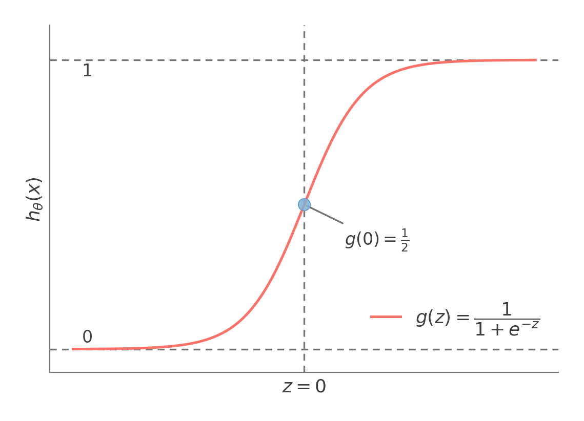
θ T x and then passes it through the sigmoid function to convert it into a value between 0 0 0 1 1 1
h θ ( x ) = g ( θ T x ) = 1 1 + e − θ T x
h_{\theta}(x)
=
g(\theta^Tx)
=
\frac{1}{
1+e^{-\theta^Tx}
}
h θ ( x ) = g ( θ T x ) = 1 + e − θ T x 1 The sigmoid function converts the score θ T x \theta^T x θ T x g ( 0 ) = 1 2 g(0)=\frac12 g ( 0 ) = 2 1
We interpret this output as the probability of class 1 1 1
p ( y = 1 ∣ x ; θ ) = h θ ( x )
p(y=1\mid x;\theta)
=
h_{\theta}(x)
p ( y = 1 ∣ x ; θ ) = h θ ( x ) and therefore:
p ( y = 0 ∣ x ; θ ) = 1 − h θ ( x )
p(y=0\mid x;\theta)
=
1-h_{\theta}(x)
p ( y = 0 ∣ x ; θ ) = 1 − h θ ( x ) Because y ∈ 0 , 1 y\in{0,1} y ∈ 0 , 1
p ( y ∣ x ; θ ) = ( h θ ( x ) ) y ( 1 − h θ ( x ) ) 1 − y
p(y\mid x;\theta)
=
\left(
h_{\theta}(x)
\right)^y
\left(
1-h_{\theta}(x)
\right)^{1-y}
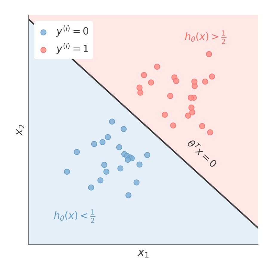
p ( y ∣ x ; θ ) = ( h θ ( x ) ) y ( 1 − h θ ( x ) ) 1 − y Logistic regression predicts one class on one side of the boundary θ T x = 0 \theta^T x = 0 θ T x = 0
Maximum-Likelihood Estimation
The log-likelihood of the training data is:
ℓ ( θ ) = log ∏ i = 1 n p ( y ( i ) ∣ x ( i ) ; θ )
\ell(\theta)
=
\log
\prod_{i=1}^{n}
p(y^{(i)}\mid x^{(i)};\theta)
ℓ ( θ ) = log i = 1 ∏ n p ( y ( i ) ∣ x ( i ) ; θ ) = ∑ i = 1 n log p ( y ( i ) ∣ x ( i ) ; θ )
=
\sum_{i=1}^{n}
\log
p(y^{(i)}\mid x^{(i)};\theta)
= i = 1 ∑ n log p ( y ( i ) ∣ x ( i ) ; θ ) = ∑ i = 1 n log [ ( h θ ( x ( i ) ) ) y ( i ) ( 1 − h θ ( x ( i ) ) ) 1 − y ( i ) ]
=
\sum_{i=1}^{n}
\log
\left[
\left(
h_{\theta}(x^{(i)})
\right)^{y^{(i)}}
\left(
1-h_{\theta}(x^{(i)})
\right)^{1-y^{(i)}}
\right]
= i = 1 ∑ n log [ ( h θ ( x ( i ) ) ) y ( i ) ( 1 − h θ ( x ( i ) ) ) 1 − y ( i ) ] Taking its derivative with respect to θ j \theta_j θ j
∂ ∂ θ j ℓ ( θ ) = ∑ i = 1 n ( y ( i ) − h θ ( x ( i ) ) ) x j ( i )
\frac{\partial}{\partial\theta_j}
\ell(\theta)
=
\sum_{i=1}^{n}
\left(
y^{(i)}
-
h_{\theta}(x^{(i)})
\right)
x_j^{(i)}
∂ θ j ∂ ℓ ( θ ) = i = 1 ∑ n ( y ( i ) − h θ ( x ( i ) ) ) x j ( i ) This is the full-data gradient.
A per-example stochastic gradient-ascent update is:
θ ← θ + α ( y ( i ) − h θ ( x ( i ) ) ) x ( i )
\theta
\leftarrow
\theta
+
\alpha
\left(
y^{(i)}
-
h_{\theta}(x^{(i)})
\right)
x^{(i)}
θ ← θ + α ( y ( i ) − h θ ( x ( i ) ) ) x ( i ) where α > 0 \alpha>0 α > 0
› See derivationFor a sigmoid function:
g ( z ) = 1 1 + e − z
g(z)
=
\frac{1}{1+e^{-z}}
g ( z ) = 1 + e − z 1 its derivative is:
d d z g ( z ) = d d z 1 1 + e − z
\frac{d}{dz}g(z)
=
\frac{d}{dz}
\frac{1}{1+e^{-z}}
d z d g ( z ) = d z d 1 + e − z 1 = d d z ( 1 + e − z ) − 1
=
\frac{d}{dz}
\left(
1+e^{-z}
\right)^{-1}
= d z d ( 1 + e − z ) − 1 = − 1 ( 1 + e − z ) − 2 ( − e − z )
=
-1
\left(
1+e^{-z}
\right)^{-2}
\left(
-e^{-z}
\right)
= − 1 ( 1 + e − z ) − 2 ( − e − z ) = 1 1 + e − z e − z 1 + e − z
=
\frac{1}{1+e^{-z}}
\frac{e^{-z}}{1+e^{-z}}
= 1 + e − z 1 1 + e − z e − z = 1 1 + e − z ( 1 − 1 1 + e − z )
=
\frac{1}{1+e^{-z}}
\left(
1-
\frac{1}{1+e^{-z}}
\right)
= 1 + e − z 1 ( 1 − 1 + e − z 1 ) = g ( z ) ( 1 − g ( z ) )
=
g(z)
\left(
1-g(z)
\right)
= g ( z ) ( 1 − g ( z ) ) ∂ ∂ θ j ℓ ( θ ) = ∂ ∂ θ j ∑ i = 1 n log [ ( h θ ( x ( i ) ) ) y ( i ) ( 1 − h θ ( x ( i ) ) ) 1 − y ( i ) ]
\frac{\partial}{\partial\theta_j}
\ell(\theta)
=
\frac{\partial}{\partial\theta_j}
\sum_{i=1}^{n}
\log
\left[
\left(
h_{\theta}(x^{(i)})
\right)^{y^{(i)}}
\left(
1-h_{\theta}(x^{(i)})
\right)^{1-y^{(i)}}
\right]
∂ θ j ∂ ℓ ( θ ) = ∂ θ j ∂ i = 1 ∑ n log [ ( h θ ( x ( i ) ) ) y ( i ) ( 1 − h θ ( x ( i ) ) ) 1 − y ( i ) ] = ∂ ∂ θ j ∑ i = 1 n ( y ( i ) log h θ ( x ( i ) ) + ( 1 − y ( i ) ) log ( 1 − h θ ( x ( i ) ) ) )
=
\frac{\partial}{\partial\theta_j}
\sum_{i=1}^{n}
\left(
y^{(i)}
\log
h_{\theta}(x^{(i)})
+
(1-y^{(i)})
\log
\left(
1-h_{\theta}(x^{(i)})
\right)
\right)
= ∂ θ j ∂ i = 1 ∑ n ( y ( i ) log h θ ( x ( i ) ) + ( 1 − y ( i ) ) log ( 1 − h θ ( x ( i ) ) ) ) = ∂ ∂ θ j ∑ i = 1 n ( y ( i ) log g ( θ T x ( i ) ) + ( 1 − y ( i ) ) log ( 1 − g ( θ T x ( i ) ) ) )
=
\frac{\partial}{\partial\theta_j}
\sum_{i=1}^{n}
\left(
y^{(i)}
\log
g(\theta^Tx^{(i)})
+
(1-y^{(i)})
\log
\left(
1-g(\theta^Tx^{(i)})
\right)
\right)
= ∂ θ j ∂ i = 1 ∑ n ( y ( i ) log g ( θ T x ( i ) ) + ( 1 − y ( i ) ) log ( 1 − g ( θ T x ( i ) ) ) ) = ∑ i = 1 n ( [ y ( i ) g ( θ T x ( i ) ) − 1 − y ( i ) 1 − g ( θ T x ( i ) ) ] ⋅ ∂ ∂ θ j [ g ( θ T x ( i ) ) ] )
=
\sum_{i=1}^{n}
\left(
\left[
\frac{y^{(i)}}{g(\theta^Tx^{(i)})}
-
\frac{1-y^{(i)}}{
1-g(\theta^Tx^{(i)})
}
\right]
\cdot
\frac{\partial}{\partial\theta_j}
\left[
g(\theta^Tx^{(i)})
\right]
\right)
= i = 1 ∑ n ( [ g ( θ T x ( i ) ) y ( i ) − 1 − g ( θ T x ( i ) ) 1 − y ( i ) ] ⋅ ∂ θ j ∂ [ g ( θ T x ( i ) ) ] ) = ∑ i = 1 n ( [ y ( i ) − g ( θ T x ( i ) ) g ( θ T x ( i ) ) ( 1 − g ( θ T x ( i ) ) ) ] ⋅ ∂ ∂ θ j [ g ( θ T x ( i ) ) ] )
=
\sum_{i=1}^{n}
\left(
\left[
\frac{
y^{(i)}-g(\theta^Tx^{(i)})
}{
g(\theta^Tx^{(i)})
\left(
1-g(\theta^Tx^{(i)})
\right)
}
\right]
\cdot
\frac{\partial}{\partial\theta_j}
\left[
g(\theta^Tx^{(i)})
\right]
\right)
= i = 1 ∑ n ( [ g ( θ T x ( i ) ) ( 1 − g ( θ T x ( i ) ) ) y ( i ) − g ( θ T x ( i ) ) ] ⋅ ∂ θ j ∂ [ g ( θ T x ( i ) ) ] ) i Using:
a b − 1 − a 1 − b = a − b b ( 1 − b )
\frac{a}{b}
-
\frac{1-a}{1-b}
=
\frac{a-b}{
b(1-b)
}
b a − 1 − b 1 − a = b ( 1 − b ) a − b = ∑ i = 1 n ( [ y ( i ) − g ( θ T x ( i ) ) g ( θ T x ( i ) ) ( 1 − g ( θ T x ( i ) ) ) ] g ( θ T x ( i ) ) ( 1 − g ( θ T x ( i ) ) ) ∂ ∂ θ j [ θ T x ( i ) ] )
=
\sum_{i=1}^{n}
\left(
\left[
\frac{
y^{(i)}-g(\theta^Tx^{(i)})
}{
g(\theta^Tx^{(i)})
\left(
1-g(\theta^Tx^{(i)})
\right)
}
\right]
g(\theta^Tx^{(i)})
\left(
1-g(\theta^Tx^{(i)})
\right)
\frac{\partial}{\partial\theta_j}
\left[
\theta^Tx^{(i)}
\right]
\right)
= i = 1 ∑ n ( [ g ( θ T x ( i ) ) ( 1 − g ( θ T x ( i ) ) ) y ( i ) − g ( θ T x ( i ) ) ] g ( θ T x ( i ) ) ( 1 − g ( θ T x ( i ) ) ) ∂ θ j ∂ [ θ T x ( i ) ] ) i Using g ′ ( z ) = g ( z ) ( 1 − g ( z ) ) g'(z)=g(z)(1-g(z)) g ′ ( z ) = g ( z ) ( 1 − g ( z ))
= ∑ i = 1 n ( y ( i ) − g ( θ T x ( i ) ) ) x j ( i )
=
\sum_{i=1}^{n}
\left(
y^{(i)}
-
g(\theta^Tx^{(i)})
\right)
x_j^{(i)}
= i = 1 ∑ n ( y ( i ) − g ( θ T x ( i ) ) ) x j ( i ) = ∑ i = 1 n ( y ( i ) − h θ ( x ( i ) ) ) x j ( i )
=
\sum_{i=1}^{n}
\left(
y^{(i)}
-
h_{\theta}(x^{(i)})
\right)
x_j^{(i)}
= i = 1 ∑ n ( y ( i ) − h θ ( x ( i ) ) ) x j ( i ) Logistic Loss
So far, we have written logistic regression as a maximum-likelihood problem.
Equivalently, we can turn it into a minimization problem by taking the negative log-likelihood.
For one example with score:
t = θ T x
t=\theta^Tx
t = θ T x the logistic loss is:
ℓ l o g i s t i c ( t , y ) = y log ( 1 + e − t ) + ( 1 − y ) log ( 1 + e t )
\ell_{\mathrm{logistic}}(t,y)
=
y
\log
\left(
1+e^{-t}
\right)
+
(1-y)
\log
\left(
1+e^t
\right)
ℓ logistic ( t , y ) = y log ( 1 + e − t ) + ( 1 − y ) log ( 1 + e t ) Therefore, maximizing the likelihood over the dataset is equivalent to minimizing the sum of these losses:
arg max θ ℓ ( θ )
\arg\max_{\theta}
\ell(\theta)
arg θ max ℓ ( θ ) = arg min θ ∑ i = 1 n ℓ l o g i s t i c ( θ T x ( i ) , y ( i ) )
=
\arg\min_{\theta}
\sum_{i=1}^{n}
\ell_{\mathrm{logistic}}
\left(
\theta^Tx^{(i)},
y^{(i)}
\right)
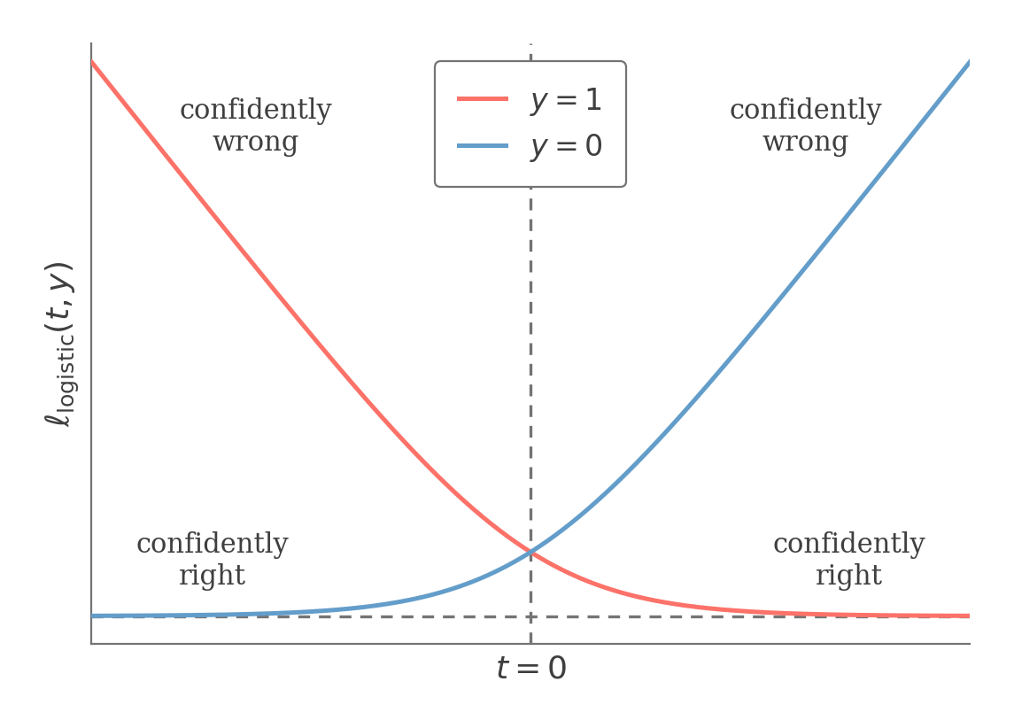
= arg θ min i = 1 ∑ n ℓ logistic ( θ T x ( i ) , y ( i ) ) Minimizing the logistic loss pushes the score t = θ T x t=\theta^Tx t = θ T x
› See derivation− log p ( y ∣ x ; θ )
-\log
p(y\mid x;\theta)
− log p ( y ∣ x ; θ ) = − y log g ( t ) − ( 1 − y ) log ( 1 − g ( t ) )
=
-y\log g(t)
-
(1-y)
\log
\left(
1-g(t)
\right)
= − y log g ( t ) − ( 1 − y ) log ( 1 − g ( t ) ) = y log ( 1 + e − t ) + ( 1 − y ) log ( 1 + e t )
=
y
\log
\left(
1+e^{-t}
\right)
+
(1-y)
\log
\left(
1+e^t
\right)
= y log ( 1 + e − t ) + ( 1 − y ) log ( 1 + e t ) = ℓ l o g i s t i c ( t , y )
=
\ell_{\mathrm{logistic}}(t,y)
= ℓ logistic ( t , y ) If the training data are completely separable, the unregularized likelihood has no finite maximizer: increasing the norm of a separating θ \theta θ
Regularization or another finite-parameter constraint prevents this divergence.
Multiclass Classification
For k k k θ j \theta_j θ j
For an input x x x j j j
θ j T x
\theta_j^Tx
θ j T x Softmax converts these k k k 1 1 1
p ( y = i ∣ x ; θ ) = ϕ i = exp ( θ i T x ) ∑ j = 1 k exp ( θ j T x )
p(y=i\mid x;\theta)
=
\phi_i
=
\frac{
\exp(\theta_i^Tx)
}{
\sum_{j=1}^{k}
\exp(\theta_j^Tx)
}
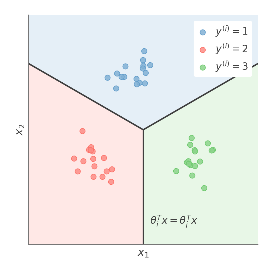
p ( y = i ∣ x ; θ ) = ϕ i = ∑ j = 1 k exp ( θ j T x ) exp ( θ i T x ) Softmax assigns each point to the class with the largest score θ i T x \theta_i^T x θ i T x k k k
Only relative class scores matter.
If the same vector a a a exp ( a T x ) \exp(a^Tx) exp ( a T x )
Consequently, the unconstrained softmax parameterization is not identifiable without fixing a reference class, imposing a constraint, or using regularization.
For each training example, we want the model to assign high probability to the correct class.
The corresponding cross-entropy loss, which is the negative log-likelihood, is:
ℓ c e ( θ ) = ∑ i = 1 m − log ( exp ( θ y ( i ) T x ( i ) ) ∑ j = 1 k exp ( θ j T x ( i ) ) )
\ell_{ce}(\theta)
=
\sum_{i=1}^{m}
-
\log
\left(
\frac{
\exp
\left(
\theta_{y^{(i)}}^Tx^{(i)}
\right)
}{
\sum_{j=1}^{k}
\exp
\left(
\theta_j^Tx^{(i)}
\right)
}
\right)
ℓ ce ( θ ) = i = 1 ∑ m − log ∑ j = 1 k exp ( θ j T x ( i ) ) exp ( θ y ( i ) T x ( i ) ) Taking the derivative of the cross-entropy loss with respect to θ j \theta_j θ j
∂ ∂ θ j ℓ c e ( θ ) = ∑ i = 1 m ( ϕ j ( i ) − 1 { y ( i ) = j } ) x ( i )
\frac{\partial}{\partial\theta_j}
\ell_{ce}(\theta)
=
\sum_{i=1}^{m}
\left(
\phi_j^{(i)}
-
1\left\{
y^{(i)}=j
\right\}
\right)
x^{(i)}
∂ θ j ∂ ℓ ce ( θ ) = i = 1 ∑ m ( ϕ j ( i ) − 1 { y ( i ) = j } ) x ( i ) where:
ϕ j ( i ) = p ( y ( i ) = j ∣ x ( i ) ; θ )
\phi_j^{(i)}
=
p
\left(
y^{(i)}=j
\mid
x^{(i)};
\theta
\right)
ϕ j ( i ) = p ( y ( i ) = j ∣ x ( i ) ; θ ) The gradient compares the model's predicted probability for class j j j
ϕ j ( i )
\phi_j^{(i)}
ϕ j ( i ) with the target:
1 { y ( i ) = j }
1\left\{
y^{(i)}=j
\right\}
1 { y ( i ) = j } In other words, the update is driven by predicted probability minus the true class indicator .
The gradient descent update is:
θ j ← θ j − α ∑ i = 1 m ( ϕ j ( i ) − 1 { y ( i ) = j } ) x ( i )
\theta_j
\leftarrow
\theta_j
-
\alpha
\sum_{i=1}^{m}
\left(
\phi_j^{(i)}
-
1\left\{
y^{(i)}=j
\right\}
\right)
x^{(i)}
θ j ← θ j − α i = 1 ∑ m ( ϕ j ( i ) − 1 { y ( i ) = j } ) x ( i ) › See derivation∂ ∂ θ l ℓ c e ( θ ) = ∂ ∂ θ l ∑ i = 1 m − log ( exp ( θ y ( i ) T x ( i ) ) ∑ j = 1 k exp ( θ j T x ( i ) ) )
\frac{\partial}{\partial\theta_l}
\ell_{ce}(\theta)
=
\frac{\partial}{\partial\theta_l}
\sum_{i=1}^{m}
-
\log
\left(
\frac{
\exp
\left(
\theta_{y^{(i)}}^Tx^{(i)}
\right)
}{
\sum_{j=1}^{k}
\exp
\left(
\theta_j^Tx^{(i)}
\right)
}
\right)
∂ θ l ∂ ℓ ce ( θ ) = ∂ θ l ∂ i = 1 ∑ m − log ∑ j = 1 k exp ( θ j T x ( i ) ) exp ( θ y ( i ) T x ( i ) ) = ∂ ∂ θ l ∑ i = 1 m [ − θ y ( i ) T x ( i ) + log ∑ j = 1 k exp ( θ j T x ( i ) ) ]
=
\frac{\partial}{\partial\theta_l}
\sum_{i=1}^{m}
\left[
-
\theta_{y^{(i)}}^Tx^{(i)}
+
\log
\sum_{j=1}^{k}
\exp
\left(
\theta_j^Tx^{(i)}
\right)
\right]
= ∂ θ l ∂ i = 1 ∑ m [ − θ y ( i ) T x ( i ) + log j = 1 ∑ k exp ( θ j T x ( i ) ) ] = ∑ i = 1 m [ ∂ ∂ θ l ( log ∑ j = 1 k exp ( θ j T x ( i ) ) ) − ∂ ∂ θ l ( θ y ( i ) T x ( i ) ) ]
=
\sum_{i=1}^{m}
\left[
\frac{\partial}{\partial\theta_l}
\left(
\log
\sum_{j=1}^{k}
\exp
\left(
\theta_j^Tx^{(i)}
\right)
\right)
-
\frac{\partial}{\partial\theta_l}
\left(
\theta_{y^{(i)}}^Tx^{(i)}
\right)
\right]
= i = 1 ∑ m [ ∂ θ l ∂ ( log j = 1 ∑ k exp ( θ j T x ( i ) ) ) − ∂ θ l ∂ ( θ y ( i ) T x ( i ) ) ] = ∑ i = 1 m [ 1 ∑ j = 1 k exp ( θ j T x ( i ) ) ( ∂ ∂ θ l ∑ j = 1 k exp ( θ j T x ( i ) ) ) − x ( i ) 1 { y ( i ) = l } ]
=
\sum_{i=1}^{m}
\left[
\frac{1}{
\sum_{j=1}^{k}
\exp
\left(
\theta_j^Tx^{(i)}
\right)
}
\left(
\frac{\partial}{\partial\theta_l}
\sum_{j=1}^{k}
\exp
\left(
\theta_j^Tx^{(i)}
\right)
\right)
-
x^{(i)}
1
\left\{
y^{(i)}=l
\right\}
\right]
= i = 1 ∑ m [ ∑ j = 1 k exp ( θ j T x ( i ) ) 1 ( ∂ θ l ∂ j = 1 ∑ k exp ( θ j T x ( i ) ) ) − x ( i ) 1 { y ( i ) = l } ] = ∑ i = 1 m [ exp ( θ l T x ( i ) ) ∑ j = 1 k exp ( θ j T x ( i ) ) x ( i ) − x ( i ) 1 { y ( i ) = l } ]
=
\sum_{i=1}^{m}
\left[
\frac{
\exp
\left(
\theta_l^Tx^{(i)}
\right)
}{
\sum_{j=1}^{k}
\exp
\left(
\theta_j^Tx^{(i)}
\right)
}
x^{(i)}
-
x^{(i)}
1
\left\{
y^{(i)}=l
\right\}
\right]
= i = 1 ∑ m [ ∑ j = 1 k exp ( θ j T x ( i ) ) exp ( θ l T x ( i ) ) x ( i ) − x ( i ) 1 { y ( i ) = l } ] = ∑ i = 1 m ( exp ( θ l T x ( i ) ) ∑ j = 1 k exp ( θ j T x ( i ) ) − 1 { y ( i ) = l } ) x ( i )
=
\sum_{i=1}^{m}
\left(
\frac{
\exp
\left(
\theta_l^Tx^{(i)}
\right)
}{
\sum_{j=1}^{k}
\exp
\left(
\theta_j^Tx^{(i)}
\right)
}
-
1
\left\{
y^{(i)}=l
\right\}
\right)
x^{(i)}
= i = 1 ∑ m ( ∑ j = 1 k exp ( θ j T x ( i ) ) exp ( θ l T x ( i ) ) − 1 { y ( i ) = l } ) x ( i ) = ∑ i = 1 m ( ϕ l ( i ) − 1 { y ( i ) = l } ) x ( i )
=
\sum_{i=1}^{m}
\left(
\phi_l^{(i)}
-
1
\left\{
y^{(i)}=l
\right\}
\right)
x^{(i)}
= i = 1 ∑ m ( ϕ l ( i ) − 1 { y ( i ) = l } ) x ( i )