Discriminative vs. Generative Models
There are two main ways to approach a classification problem.
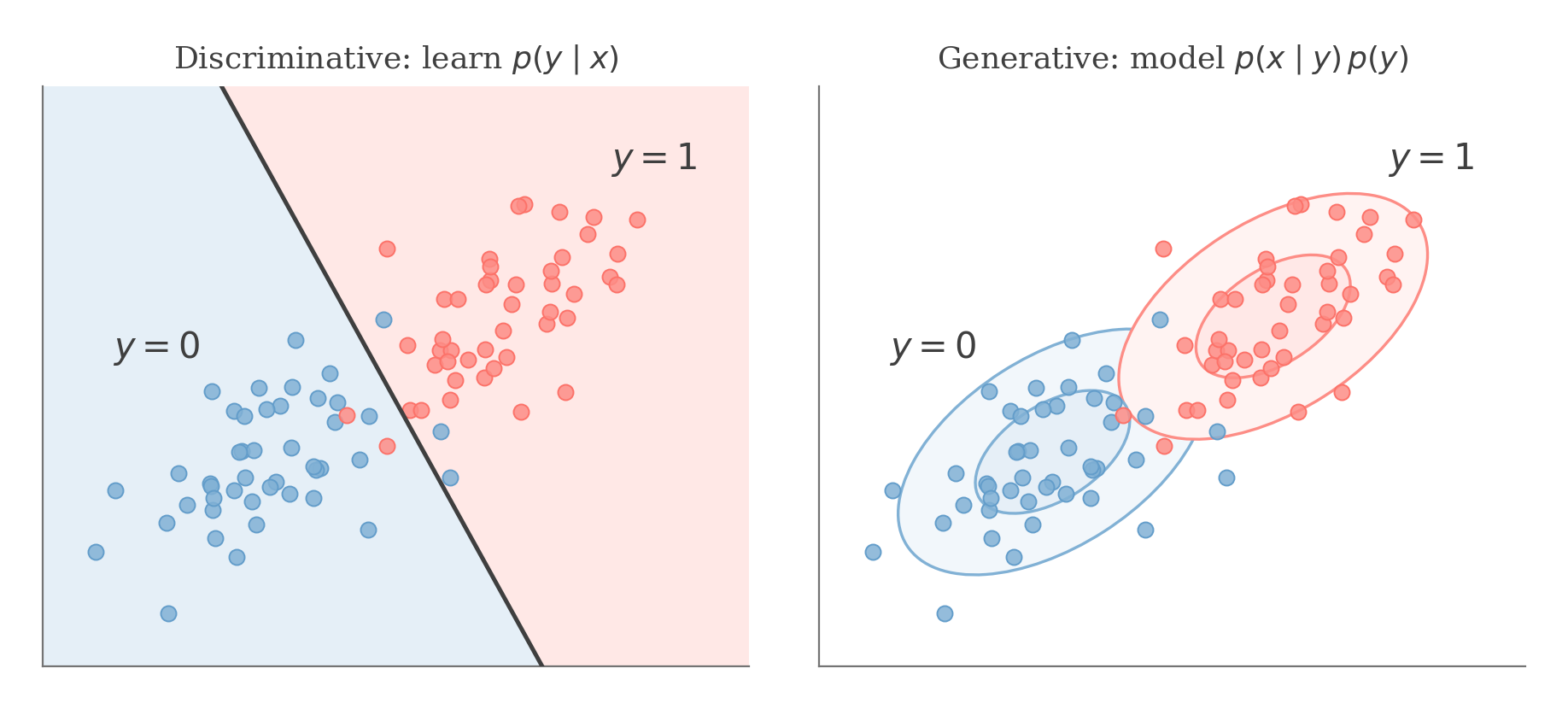
A discriminative model learns to predict the class directly from the input. In probabilistic terms, it models:
p ( y ∣ x )
p(y \mid x)
p ( y ∣ x ) A generative model takes a different approach. It learns how the input is distributed within each class by modelling:
p ( x ∣ y )
p(x \mid y)
p ( x ∣ y ) along with the class probabilities:
p ( y )
p(y)
p ( y ) A discriminative model focuses on separating the classes directly, while a generative model first models what the data from each class looks like.
Once we know p ( x ∣ y ) p(x \mid y) p ( x ∣ y ) p ( y ) p(y) p ( y ) p ( y ∣ x ) p(y \mid x) p ( y ∣ x )
arg max y p ( y ∣ x ) = arg max y p ( x ∣ y ) p ( y ) p ( x )
\arg \max_y p(y \mid x)
=
\arg \max_y \frac{p(x \mid y)p(y)}{p(x)}
arg y max p ( y ∣ x ) = arg y max p ( x ) p ( x ∣ y ) p ( y ) = arg max y p ( x ∣ y ) p ( y )
= \arg \max_y p(x \mid y)p(y)
= arg y max p ( x ∣ y ) p ( y ) The denominator p ( x ) p(x) p ( x ) p ( x ∣ y ) p ( y ) p(x \mid y)p(y) p ( x ∣ y ) p ( y )
Gaussian Discriminant Analysis
Gaussian Discriminant Analysis (GDA) makes this generative approach concrete by assuming that the inputs from each class follow a Gaussian distribution.
For binary classification, let:
y ∈ { 0 , 1 } , x ∈ R d
y \in \{0,1\},
\qquad
x \in \mathbb{R}^d
y ∈ { 0 , 1 } , x ∈ R d We model the class prior using a parameter ϕ \phi ϕ
p ( y ) = ϕ y ( 1 − ϕ ) 1 − y
p(y) = \phi^y(1-\phi)^{1-y}
p ( y ) = ϕ y ( 1 − ϕ ) 1 − y Each class has its own mean:
μ 0 , μ 1
\mu_0,
\qquad
\mu_1
μ 0 , μ 1 but both classes share the same covariance matrix Σ \Sigma Σ
Therefore:
x ∣ y = 0 ∼ N ( μ 0 , Σ )
x \mid y=0 \sim \mathcal{N}(\mu_0,\Sigma)
x ∣ y = 0 ∼ N ( μ 0 , Σ ) x ∣ y = 1 ∼ N ( μ 1 , Σ )
x \mid y=1 \sim \mathcal{N}(\mu_1,\Sigma)
x ∣ y = 1 ∼ N ( μ 1 , Σ ) The corresponding densities are:
p ( x ∣ y = 0 ) = 1 ( 2 π ) d / 2 ∣ Σ ∣ 1 / 2 exp ( − 1 2 ( x − μ 0 ) T Σ − 1 ( x − μ 0 ) )
p(x \mid y = 0)
=
\frac{1}{(2 \pi)^{d/2} |\Sigma|^{1/2}}
\exp \left(
-\frac{1}{2}
(x-\mu_0)^T
\Sigma^{-1}
(x-\mu_0)
\right)
p ( x ∣ y = 0 ) = ( 2 π ) d /2 ∣Σ ∣ 1/2 1 exp ( − 2 1 ( x − μ 0 ) T Σ − 1 ( x − μ 0 ) ) p ( x ∣ y = 1 ) = 1 ( 2 π ) d / 2 ∣ Σ ∣ 1 / 2 exp ( − 1 2 ( x − μ 1 ) T Σ − 1 ( x − μ 1 ) )
p(x \mid y = 1)
=
\frac{1}{(2 \pi)^{d/2} |\Sigma|^{1/2}}
\exp \left(
-\frac{1}{2}
(x-\mu_1)^T
\Sigma^{-1}
(x-\mu_1)
\right)
p ( x ∣ y = 1 ) = ( 2 π ) d /2 ∣Σ ∣ 1/2 1 exp ( − 2 1 ( x − μ 1 ) T Σ − 1 ( x − μ 1 ) ) GDA therefore has four quantities to learn from the training data:
ϕ , μ 0 , μ 1 , Σ
\phi,
\qquad
\mu_0,
\qquad
\mu_1,
\qquad
\Sigma
ϕ , μ 0 , μ 1 , Σ Maximum-Likelihood Estimation
We estimate them by maximizing the likelihood of the observed training data.
The log-likelihood is:
ℓ ( ϕ , μ 0 , μ 1 , Σ ) = log ∏ i = 1 n p ( x ( i ) , y ( i ) ; ϕ , μ 0 , μ 1 , Σ )
\ell(\phi,\mu_0,\mu_1,\Sigma)
=
\log
\prod_{i=1}^n
p\left(
x^{(i)},y^{(i)};
\phi,\mu_0,\mu_1,\Sigma
\right)
ℓ ( ϕ , μ 0 , μ 1 , Σ ) = log i = 1 ∏ n p ( x ( i ) , y ( i ) ; ϕ , μ 0 , μ 1 , Σ ) Maximizing this log-likelihood gives:
ϕ = 1 n ∑ i = 1 n 1 { y ( i ) = 1 }
\phi
=
\frac{1}{n}
\sum_{i=1}^n
1\left\{y^{(i)}=1\right\}
ϕ = n 1 i = 1 ∑ n 1 { y ( i ) = 1 } μ 0 = ∑ i = 1 n 1 { y ( i ) = 0 } x ( i ) ∑ i = 1 n 1 { y ( i ) = 0 }
\mu_0
=
\frac{
\sum_{i=1}^n
1\left\{y^{(i)}=0\right\}x^{(i)}
}{
\sum_{i=1}^n
1\left\{y^{(i)}=0\right\}
}
μ 0 = ∑ i = 1 n 1 { y ( i ) = 0 } ∑ i = 1 n 1 { y ( i ) = 0 } x ( i ) μ 1 = ∑ i = 1 n 1 { y ( i ) = 1 } x ( i ) ∑ i = 1 n 1 { y ( i ) = 1 }
\mu_1
=
\frac{
\sum_{i=1}^n
1\left\{y^{(i)}=1\right\}x^{(i)}
}{
\sum_{i=1}^n
1\left\{y^{(i)}=1\right\}
}
μ 1 = ∑ i = 1 n 1 { y ( i ) = 1 } ∑ i = 1 n 1 { y ( i ) = 1 } x ( i ) Σ = 1 n ∑ i = 1 n ( x ( i ) − μ y ( i ) ) ( x ( i ) − μ y ( i ) ) T
\Sigma
=
\frac{1}{n}
\sum_{i=1}^n
\left(
x^{(i)}-\mu_{y^{(i)}}
\right)
\left(
x^{(i)}-\mu_{y^{(i)}}
\right)^T
Σ = n 1 i = 1 ∑ n ( x ( i ) − μ y ( i ) ) ( x ( i ) − μ y ( i ) ) T These estimates have a simple interpretation.
ϕ \phi ϕ 1 1 1
μ 0 \mu_0 μ 0 0 0 0 μ 1 \mu_1 μ 1 1 1 1
Σ \Sigma Σ
Once these parameters are fitted, prediction is straightforward. For a new input x x x
p ( x ∣ y = 0 ) p ( y = 0 )
p(x \mid y=0)p(y=0)
p ( x ∣ y = 0 ) p ( y = 0 ) and
p ( x ∣ y = 1 ) p ( y = 1 )
p(x \mid y=1)p(y=1)
p ( x ∣ y = 1 ) p ( y = 1 ) and choose whichever is larger.
Because both classes use the same covariance matrix, the quadratic terms cancel when we compare their log probabilities. This is why the resulting decision boundary is linear.
The formulas above assume that both classes appear in the training set and that the pooled covariance matrix is nonsingular. If the covariance is singular, a common practical approach is to regularize it, for example by replacing Σ \Sigma Σ
Σ + λ I
\Sigma + \lambda I
Σ + λ I for some λ > 0 \lambda > 0 λ > 0
› See derivationWe start with the log-likelihood:
ℓ ( ϕ , μ 0 , μ 1 , Σ ) = log ∏ i = 1 n p ( x ( i ) , y ( i ) ; ϕ , μ 0 , μ 1 , Σ )
\ell(\phi,\mu_0,\mu_1,\Sigma)
=
\log
\prod_{i=1}^n
p\left(
x^{(i)},y^{(i)};
\phi,\mu_0,\mu_1,\Sigma
\right)
ℓ ( ϕ , μ 0 , μ 1 , Σ ) = log i = 1 ∏ n p ( x ( i ) , y ( i ) ; ϕ , μ 0 , μ 1 , Σ ) = log ∏ i = 1 n p ( x ( i ) ∣ y ( i ) ; μ y ( i ) , Σ ) p ( y ( i ) ; ϕ )
=
\log
\prod_{i=1}^n
p(x^{(i)}\mid y^{(i)};\mu_{y^{(i)}},\Sigma)
p(y^{(i)};\phi)
= log i = 1 ∏ n p ( x ( i ) ∣ y ( i ) ; μ y ( i ) , Σ ) p ( y ( i ) ; ϕ ) i Using the factorization p ( x , y ) = p ( x ∣ y ) p ( y ) p(x,y)=p(x\mid y)p(y) p ( x , y ) = p ( x ∣ y ) p ( y )
Taking the log of the product gives:
= ∑ i = 1 n [ y ( i ) log p ( x ( i ) ∣ y ( i ) = 1 ; μ 1 , Σ ) + ( 1 − y ( i ) ) log p ( x ( i ) ∣ y ( i ) = 0 ; μ 0 , Σ )
=
\sum_{i=1}^n
\left[
y^{(i)}
\log
p(x^{(i)}\mid y^{(i)}=1;\mu_1,\Sigma)
+
(1-y^{(i)})
\log
p(x^{(i)}\mid y^{(i)}=0;\mu_0,\Sigma)
\right.
= i = 1 ∑ n [ y ( i ) log p ( x ( i ) ∣ y ( i ) = 1 ; μ 1 , Σ ) + ( 1 − y ( i ) ) log p ( x ( i ) ∣ y ( i ) = 0 ; μ 0 , Σ ) + y ( i ) log ϕ + ( 1 − y ( i ) ) log ( 1 − ϕ ) ]
\left.
+
y^{(i)}\log\phi
+
(1-y^{(i)})\log(1-\phi)
\right]
+ y ( i ) log ϕ + ( 1 − y ( i ) ) log ( 1 − ϕ ) ] First, take the derivative with respect to ϕ \phi ϕ
∇ ϕ ℓ = ∑ i = 1 n ( y ( i ) ϕ − 1 − y ( i ) 1 − ϕ )
\nabla_\phi \ell
=
\sum_{i=1}^n
\left(
\frac{y^{(i)}}{\phi}
-
\frac{1-y^{(i)}}{1-\phi}
\right)
∇ ϕ ℓ = i = 1 ∑ n ( ϕ y ( i ) − 1 − ϕ 1 − y ( i ) ) = ∑ i = 1 n y ( i ) − ϕ ϕ ( 1 − ϕ )
=
\sum_{i=1}^n
\frac{y^{(i)}-\phi}{\phi(1-\phi)}
= i = 1 ∑ n ϕ ( 1 − ϕ ) y ( i ) − ϕ i Combining the two fractions over a common denominator.
Setting the derivative equal to 0 0 0
∑ i = 1 n ( y ( i ) − ϕ ) = 0
\sum_{i=1}^n
\left(
y^{(i)}-\phi
\right)
=
0
i = 1 ∑ n ( y ( i ) − ϕ ) = 0 Therefore:
ϕ = 1 n ∑ i = 1 n y ( i )
\phi
=
\frac{1}{n}
\sum_{i=1}^n y^{(i)}
ϕ = n 1 i = 1 ∑ n y ( i ) ϕ = 1 n ∑ i = 1 n 1 { y ( i ) = 1 }
\phi
=
\frac{1}{n}
\sum_{i=1}^n
1\left\{y^{(i)}=1\right\}
ϕ = n 1 i = 1 ∑ n 1 { y ( i ) = 1 } Now take the derivative with respect to μ 0 \mu_0 μ 0 0 0 0 μ 0 \mu_0 μ 0
∇ μ 0 ℓ = ∇ μ 0 ∑ i = 1 n ( 1 − y ( i ) ) [ − 1 2 ( x ( i ) − μ 0 ) T Σ − 1 ( x ( i ) − μ 0 ) ]
\nabla_{\mu_0}\ell
=
\nabla_{\mu_0}
\sum_{i=1}^n
(1-y^{(i)})
\left[
-\frac{1}{2}
(x^{(i)}-\mu_0)^T
\Sigma^{-1}
(x^{(i)}-\mu_0)
\right]
∇ μ 0 ℓ = ∇ μ 0 i = 1 ∑ n ( 1 − y ( i ) ) [ − 2 1 ( x ( i ) − μ 0 ) T Σ − 1 ( x ( i ) − μ 0 ) ] = ∑ i = 1 n ( 1 − y ( i ) ) Σ − 1 ( x ( i ) − μ 0 )
=
\sum_{i=1}^n
(1-y^{(i)})
\Sigma^{-1}
\left(
x^{(i)}-\mu_0
\right)
= i = 1 ∑ n ( 1 − y ( i ) ) Σ − 1 ( x ( i ) − μ 0 ) i Using ∇ μ [ − 1 2 ( x − μ ) T A ( x − μ ) ] = A ( x − μ ) \nabla_\mu\left[-\frac12(x-\mu)^TA(x-\mu)\right]=A(x-\mu) ∇ μ [ − 2 1 ( x − μ ) T A ( x − μ ) ] = A ( x − μ ) A A A
Setting this equal to 0 0 0
∑ i = 1 n ( 1 − y ( i ) ) Σ − 1 ( x ( i ) − μ 0 ) = 0
\sum_{i=1}^n
(1-y^{(i)})
\Sigma^{-1}
\left(
x^{(i)}-\mu_0
\right)
=
0
i = 1 ∑ n ( 1 − y ( i ) ) Σ − 1 ( x ( i ) − μ 0 ) = 0 ∑ i = 1 n ( 1 − y ( i ) ) x ( i ) = [ ∑ i = 1 n ( 1 − y ( i ) ) ] μ 0
\sum_{i=1}^n
(1-y^{(i)})
x^{(i)}
=
\left[
\sum_{i=1}^n
(1-y^{(i)})
\right]\mu_0
i = 1 ∑ n ( 1 − y ( i ) ) x ( i ) = [ i = 1 ∑ n ( 1 − y ( i ) ) ] μ 0 i Σ − 1 \Sigma^{-1} Σ − 1 i i i
Therefore:
μ 0 = ∑ i = 1 n ( 1 − y ( i ) ) x ( i ) ∑ i = 1 n ( 1 − y ( i ) )
\mu_0
=
\frac{
\sum_{i=1}^n
(1-y^{(i)})x^{(i)}
}{
\sum_{i=1}^n
(1-y^{(i)})
}
μ 0 = ∑ i = 1 n ( 1 − y ( i ) ) ∑ i = 1 n ( 1 − y ( i ) ) x ( i ) μ 0 = ∑ i = 1 n 1 { y ( i ) = 0 } x ( i ) ∑ i = 1 n 1 { y ( i ) = 0 }
\mu_0
=
\frac{
\sum_{i=1}^n
1\left\{y^{(i)}=0\right\}x^{(i)}
}{
\sum_{i=1}^n
1\left\{y^{(i)}=0\right\}
}
μ 0 = ∑ i = 1 n 1 { y ( i ) = 0 } ∑ i = 1 n 1 { y ( i ) = 0 } x ( i ) Similarly:
μ 1 = ∑ i = 1 n 1 { y ( i ) = 1 } x ( i ) ∑ i = 1 n 1 { y ( i ) = 1 }
\mu_1
=
\frac{
\sum_{i=1}^n
1\left\{y^{(i)}=1\right\}x^{(i)}
}{
\sum_{i=1}^n
1\left\{y^{(i)}=1\right\}
}
μ 1 = ∑ i = 1 n 1 { y ( i ) = 1 } ∑ i = 1 n 1 { y ( i ) = 1 } x ( i ) Finally, take the derivative with respect to Σ \Sigma Σ
For an invertible matrix A A A
∇ A log ∣ A ∣ = A − T
\nabla_A \log |A|
=
A^{-T}
∇ A log ∣ A ∣ = A − T and
∇ A ( x T A − 1 x ) = − A − T x x T A − T
\nabla_A
\left(
x^T A^{-1}x
\right)
=
-A^{-T}xx^TA^{-T}
∇ A ( x T A − 1 x ) = − A − T x x T A − T When A A A
A − T = A − 1
A^{-T}=A^{-1}
A − T = A − 1 For one Gaussian term, the parts that depend on Σ \Sigma Σ
− 1 2 log ∣ Σ ∣ − 1 2 ( x − μ ) T Σ − 1 ( x − μ )
-\frac{1}{2}\log|\Sigma|
-
\frac{1}{2}
(x-\mu)^T
\Sigma^{-1}
(x-\mu)
− 2 1 log ∣Σ∣ − 2 1 ( x − μ ) T Σ − 1 ( x − μ ) Differentiating gives:
− 1 2 Σ − 1 + 1 2 Σ − 1 ( x − μ ) ( x − μ ) T Σ − 1
-\frac{1}{2}\Sigma^{-1}
+
\frac{1}{2}
\Sigma^{-1}
(x-\mu)(x-\mu)^T
\Sigma^{-1}
− 2 1 Σ − 1 + 2 1 Σ − 1 ( x − μ ) ( x − μ ) T Σ − 1 i Using the derivative of log ∣ Σ ∣ \log|\Sigma| log ∣Σ∣ Σ − 1 \Sigma^{-1} Σ − 1
Applying this to every training example:
∇ Σ ℓ = 1 2 ∑ i = 1 n [ − Σ − 1 + Σ − 1 ( x ( i ) − μ y ( i ) ) ( x ( i ) − μ y ( i ) ) T Σ − 1 ]
\nabla_\Sigma \ell
=
\frac{1}{2}
\sum_{i=1}^n
\left[
-\Sigma^{-1}
+
\Sigma^{-1}
\left(
x^{(i)}-\mu_{y^{(i)}}
\right)
\left(
x^{(i)}-\mu_{y^{(i)}}
\right)^T
\Sigma^{-1}
\right]
∇ Σ ℓ = 2 1 i = 1 ∑ n [ − Σ − 1 + Σ − 1 ( x ( i ) − μ y ( i ) ) ( x ( i ) − μ y ( i ) ) T Σ − 1 ] Setting this equal to 0 0 0
∑ i = 1 n [ − Σ − 1 + Σ − 1 ( x ( i ) − μ y ( i ) ) ( x ( i ) − μ y ( i ) ) T Σ − 1 ] = 0
\sum_{i=1}^n
\left[
-\Sigma^{-1}
+
\Sigma^{-1}
\left(
x^{(i)}-\mu_{y^{(i)}}
\right)
\left(
x^{(i)}-\mu_{y^{(i)}}
\right)^T
\Sigma^{-1}
\right]
=
0
i = 1 ∑ n [ − Σ − 1 + Σ − 1 ( x ( i ) − μ y ( i ) ) ( x ( i ) − μ y ( i ) ) T Σ − 1 ] = 0 n Σ − 1 = Σ − 1 [ ∑ i = 1 n ( x ( i ) − μ y ( i ) ) ( x ( i ) − μ y ( i ) ) T ] Σ − 1
n\Sigma^{-1}
=
\Sigma^{-1}
\left[
\sum_{i=1}^n
\left(
x^{(i)}-\mu_{y^{(i)}}
\right)
\left(
x^{(i)}-\mu_{y^{(i)}}
\right)^T
\right]
\Sigma^{-1}
n Σ − 1 = Σ − 1 [ i = 1 ∑ n ( x ( i ) − μ y ( i ) ) ( x ( i ) − μ y ( i ) ) T ] Σ − 1 i Σ − 1 \Sigma^{-1} Σ − 1 i i i
Multiplying on both sides by Σ \Sigma Σ
Σ = 1 n ∑ i = 1 n ( x ( i ) − μ y ( i ) ) ( x ( i ) − μ y ( i ) ) T
\Sigma
=
\frac{1}{n}
\sum_{i=1}^n
\left(
x^{(i)}-\mu_{y^{(i)}}
\right)
\left(
x^{(i)}-\mu_{y^{(i)}}
\right)^T
Σ = n 1 i = 1 ∑ n ( x ( i ) − μ y ( i ) ) ( x ( i ) − μ y ( i ) ) T Naive Bayes
GDA models the entire feature vector x x x
Naive Bayes takes a simpler approach: it assumes that the features are conditionally independent once we know the class.
For binary features, this gives Bernoulli Naive Bayes .
We assume:
x ∈ { 0 , 1 } d
x \in \{0,1\}^d
x ∈ { 0 , 1 } d and:
p ( x 1 , … , x d ∣ y ) = ∏ j = 1 d p ( x j ∣ y )
p(x_1,\ldots,x_d\mid y)
=
\prod_{j=1}^d p(x_j\mid y)
p ( x 1 , … , x d ∣ y ) = j = 1 ∏ d p ( x j ∣ y ) In words, once we know the class y y y
This assumption is usually not exactly true, which is why the model is called "naive." However, it makes the model very simple to estimate.
For each feature j j j
ϕ j ∣ y = 1 = p ( x j = 1 ∣ y = 1 )
\phi_{j\mid y=1}
=
p(x_j=1\mid y=1)
ϕ j ∣ y = 1 = p ( x j = 1 ∣ y = 1 ) and:
ϕ j ∣ y = 0 = p ( x j = 1 ∣ y = 0 )
\phi_{j\mid y=0}
=
p(x_j=1\mid y=0)
ϕ j ∣ y = 0 = p ( x j = 1 ∣ y = 0 ) We also use:
ϕ y = p ( y = 1 )
\phi_y
=
p(y=1)
ϕ y = p ( y = 1 ) for the class prior.
For binary classification:
y ∈ { 0 , 1 }
y\in\{0,1\}
y ∈ { 0 , 1 } Because of the conditional-independence assumption, the probability of an entire feature vector factors into a product of simple probabilities.
The log-likelihood is:
ℓ ( ϕ y , ϕ j ∣ y = 0 , ϕ j ∣ y = 1 ) = log ∏ i = 1 n p ( x ( i ) , y ( i ) ; ϕ y , ϕ j ∣ y = 0 , ϕ j ∣ y = 1 )
\ell(
\phi_y,
\phi_{j\mid y=0},
\phi_{j\mid y=1}
)
=
\log
\prod_{i=1}^n
p\left(
x^{(i)},y^{(i)};
\phi_y,
\phi_{j\mid y=0},
\phi_{j\mid y=1}
\right)
ℓ ( ϕ y , ϕ j ∣ y = 0 , ϕ j ∣ y = 1 ) = log i = 1 ∏ n p ( x ( i ) , y ( i ) ; ϕ y , ϕ j ∣ y = 0 , ϕ j ∣ y = 1 ) Using the Naive Bayes factorization:
= log ∏ i = 1 n ( ∏ j = 1 d p ( x j ( i ) ∣ y ( i ) ) ) p ( y ( i ) )
=
\log
\prod_{i=1}^n
\left(
\prod_{j=1}^d
p(
x_j^{(i)}
\mid
y^{(i)}
)
\right)
p(y^{(i)})
= log i = 1 ∏ n ( j = 1 ∏ d p ( x j ( i ) ∣ y ( i ) ) ) p ( y ( i ) ) Maximizing the log-likelihood gives:
ϕ j ∣ y = 1 = ∑ i = 1 n 1 { x j ( i ) = 1 ∧ y ( i ) = 1 } ∑ i = 1 n 1 { y ( i ) = 1 }
\phi_{j\mid y=1}
=
\frac{
\sum_{i=1}^{n}
1\left\{
x_j^{(i)}=1
\land
y^{(i)}=1
\right\}
}{
\sum_{i=1}^{n}
1\left\{
y^{(i)}=1
\right\}
}
ϕ j ∣ y = 1 = ∑ i = 1 n 1 { y ( i ) = 1 } ∑ i = 1 n 1 { x j ( i ) = 1 ∧ y ( i ) = 1 } ϕ j ∣ y = 0 = ∑ i = 1 n 1 { x j ( i ) = 1 ∧ y ( i ) = 0 } ∑ i = 1 n 1 { y ( i ) = 0 }
\phi_{j\mid y=0}
=
\frac{
\sum_{i=1}^{n}
1\left\{
x_j^{(i)}=1
\land
y^{(i)}=0
\right\}
}{
\sum_{i=1}^{n}
1\left\{
y^{(i)}=0
\right\}
}
ϕ j ∣ y = 0 = ∑ i = 1 n 1 { y ( i ) = 0 } ∑ i = 1 n 1 { x j ( i ) = 1 ∧ y ( i ) = 0 } ϕ y = 1 n ∑ i = 1 n 1 { y ( i ) = 1 }
\phi_y
=
\frac{1}{n}
\sum_{i=1}^{n}
1\left\{
y^{(i)}=1
\right\}
ϕ y = n 1 i = 1 ∑ n 1 { y ( i ) = 1 } Again, these estimates are just empirical frequencies.
For example,
ϕ j ∣ y = 1
\phi_{j\mid y=1}
ϕ j ∣ y = 1 is the fraction of class-1 1 1 j j j 1 1 1
Similarly,
ϕ j ∣ y = 0
\phi_{j\mid y=0}
ϕ j ∣ y = 0 is the fraction of class-0 0 0 j j j 1 1 1
Prediction
To classify a new input x x x
Using Bayes' rule:
p ( y = 1 ∣ x ) = p ( x ∣ y = 1 ) p ( y = 1 ) p ( x )
p(y=1\mid x)
=
\frac{
p(x\mid y=1)p(y=1)
}{
p(x)
}
p ( y = 1 ∣ x ) = p ( x ) p ( x ∣ y = 1 ) p ( y = 1 ) Because of the conditional-independence assumption:
p ( x ∣ y = 1 ) = ∏ j = 1 d p ( x j ∣ y = 1 )
p(x\mid y=1)
=
\prod_{j=1}^{d}
p(x_j\mid y=1)
p ( x ∣ y = 1 ) = j = 1 ∏ d p ( x j ∣ y = 1 ) Therefore:
p ( y = 1 ∣ x ) = ( ∏ j = 1 d p ( x j ∣ y = 1 ) ) p ( y = 1 ) ( ∏ j = 1 d p ( x j ∣ y = 1 ) ) p ( y = 1 ) + ( ∏ j = 1 d p ( x j ∣ y = 0 ) ) p ( y = 0 )
p(y=1\mid x)
=
\frac{
\left(
\prod_{j=1}^{d}
p(x_j\mid y=1)
\right)
p(y=1)
}{
\left(
\prod_{j=1}^{d}
p(x_j\mid y=1)
\right)
p(y=1)
+
\left(
\prod_{j=1}^{d}
p(x_j\mid y=0)
\right)
p(y=0)
}
p ( y = 1 ∣ x ) = ( ∏ j = 1 d p ( x j ∣ y = 1 ) ) p ( y = 1 ) + ( ∏ j = 1 d p ( x j ∣ y = 0 ) ) p ( y = 0 ) ( ∏ j = 1 d p ( x j ∣ y = 1 ) ) p ( y = 1 ) For classification alone, we do not actually need to calculate the denominator. It is the same for both classes.
We can simply compare:
p ( x ∣ y = 1 ) p ( y = 1 )
p(x\mid y=1)p(y=1)
p ( x ∣ y = 1 ) p ( y = 1 ) and
p ( x ∣ y = 0 ) p ( y = 0 )
p(x\mid y=0)p(y=0)
p ( x ∣ y = 0 ) p ( y = 0 ) and choose whichever is larger.
Laplace Smoothing
There is one important problem with estimating the probabilities using raw counts.
Suppose feature j j j 1 1 1
p ( x j = 1 ∣ y = 1 ) = 0
p(x_j=1\mid y=1)=0
p ( x j = 1 ∣ y = 1 ) = 0 Naive Bayes multiplies the feature probabilities together, so this single zero can make the probability of the entire input under class 1 1 1
Laplace smoothing avoids this by pretending that we have seen each possible binary outcome once before observing the training data.
We therefore add one pseudocount to each outcome:
ϕ j ∣ y = 1 = 1 + ∑ i = 1 n 1 { x j ( i ) = 1 ∧ y ( i ) = 1 } 2 + ∑ i = 1 n 1 { y ( i ) = 1 }
\phi_{j\mid y=1}
=
\frac{
1+
\sum_{i=1}^{n}
1\left\{
x_j^{(i)}=1
\land
y^{(i)}=1
\right\}
}{
2+
\sum_{i=1}^{n}
1\left\{
y^{(i)}=1
\right\}
}
ϕ j ∣ y = 1 = 2 + ∑ i = 1 n 1 { y ( i ) = 1 } 1 + ∑ i = 1 n 1 { x j ( i ) = 1 ∧ y ( i ) = 1 } ϕ j ∣ y = 0 = 1 + ∑ i = 1 n 1 { x j ( i ) = 1 ∧ y ( i ) = 0 } 2 + ∑ i = 1 n 1 { y ( i ) = 0 }
\phi_{j\mid y=0}
=
\frac{
1+
\sum_{i=1}^{n}
1\left\{
x_j^{(i)}=1
\land
y^{(i)}=0
\right\}
}{
2+
\sum_{i=1}^{n}
1\left\{
y^{(i)}=0
\right\}
}
ϕ j ∣ y = 0 = 2 + ∑ i = 1 n 1 { y ( i ) = 0 } 1 + ∑ i = 1 n 1 { x j ( i ) = 1 ∧ y ( i ) = 0 } The class prior remains:
ϕ y = 1 n ∑ i = 1 n 1 { y ( i ) = 1 }
\phi_y
=
\frac{1}{n}
\sum_{i=1}^{n}
1\left\{
y^{(i)}=1
\right\}
ϕ y = n 1 i = 1 ∑ n 1 { y ( i ) = 1 } The added pseudocounts prevent a feature probability from becoming exactly 0 0 0 1 1 1
› See derivationThe log-likelihood is:
ℓ ( ϕ y , ϕ j ∣ y = 0 , ϕ j ∣ y = 1 ) = log ∏ i = 1 n ( ∏ j = 1 d p ( x j ( i ) ∣ y ( i ) ) ) p ( y ( i ) )
\ell(
\phi_y,
\phi_{j\mid y=0},
\phi_{j\mid y=1}
)
=
\log
\prod_{i=1}^n
\left(
\prod_{j=1}^d
p(
x_j^{(i)}
\mid
y^{(i)}
)
\right)
p(y^{(i)})
ℓ ( ϕ y , ϕ j ∣ y = 0 , ϕ j ∣ y = 1 ) = log i = 1 ∏ n ( j = 1 ∏ d p ( x j ( i ) ∣ y ( i ) ) ) p ( y ( i ) ) For binary features and labels, this becomes:
= ∑ i = 1 n [ ∑ j = 1 d ( x j ( i ) y ( i ) log ϕ j ∣ y = 1
=
\sum_{i=1}^n
\left[
\sum_{j=1}^d
\left(
x_j^{(i)}y^{(i)}
\log\phi_{j\mid y=1}
\right.
\right.
= i = 1 ∑ n [ j = 1 ∑ d ( x j ( i ) y ( i ) log ϕ j ∣ y = 1 + ( 1 − x j ( i ) ) y ( i ) log ( 1 − ϕ j ∣ y = 1 )
+
(1-x_j^{(i)})y^{(i)}
\log(1-\phi_{j\mid y=1})
+ ( 1 − x j ( i ) ) y ( i ) log ( 1 − ϕ j ∣ y = 1 ) + x j ( i ) ( 1 − y ( i ) ) log ϕ j ∣ y = 0
+
x_j^{(i)}(1-y^{(i)})
\log\phi_{j\mid y=0}
+ x j ( i ) ( 1 − y ( i ) ) log ϕ j ∣ y = 0 + ( 1 − x j ( i ) ) ( 1 − y ( i ) ) log ( 1 − ϕ j ∣ y = 0 ) )
\left.
+
(1-x_j^{(i)})(1-y^{(i)})
\log(1-\phi_{j\mid y=0})
\right)
+ ( 1 − x j ( i ) ) ( 1 − y ( i ) ) log ( 1 − ϕ j ∣ y = 0 ) ) + y ( i ) log ϕ y + ( 1 − y ( i ) ) log ( 1 − ϕ y ) ]
\left.
+
y^{(i)}\log\phi_y
+
(1-y^{(i)})\log(1-\phi_y)
\right]
+ y ( i ) log ϕ y + ( 1 − y ( i ) ) log ( 1 − ϕ y ) ] First, take the derivative with respect to ϕ y \phi_y ϕ y
∇ ϕ y ℓ = ∑ i = 1 n ( y ( i ) ϕ y − 1 − y ( i ) 1 − ϕ y )
\nabla_{\phi_y}\ell
=
\sum_{i=1}^n
\left(
\frac{y^{(i)}}{\phi_y}
-
\frac{1-y^{(i)}}{1-\phi_y}
\right)
∇ ϕ y ℓ = i = 1 ∑ n ( ϕ y y ( i ) − 1 − ϕ y 1 − y ( i ) ) = ∑ i = 1 n y ( i ) − ϕ y ϕ y ( 1 − ϕ y )
=
\sum_{i=1}^n
\frac{y^{(i)}-\phi_y}
{\phi_y(1-\phi_y)}
= i = 1 ∑ n ϕ y ( 1 − ϕ y ) y ( i ) − ϕ y i Combining the two fractions over a common denominator.
Setting this equal to 0 0 0
∑ i = 1 n ( y ( i ) − ϕ y ) = 0
\sum_{i=1}^n
\left(
y^{(i)}-\phi_y
\right)
=
0
i = 1 ∑ n ( y ( i ) − ϕ y ) = 0 Therefore:
ϕ y = 1 n ∑ i = 1 n y ( i )
\phi_y
=
\frac{1}{n}
\sum_{i=1}^n
y^{(i)}
ϕ y = n 1 i = 1 ∑ n y ( i ) ϕ y = 1 n ∑ i = 1 n 1 { y ( i ) = 1 }
\phi_y
=
\frac{1}{n}
\sum_{i=1}^n
1\left\{
y^{(i)}=1
\right\}
ϕ y = n 1 i = 1 ∑ n 1 { y ( i ) = 1 } Now take the derivative with respect to ϕ k ∣ y = 1 \phi_{k\mid y=1} ϕ k ∣ y = 1
∇ ϕ k ∣ y = 1 ℓ = ∑ i = 1 n [ x k ( i ) y ( i ) ϕ k ∣ y = 1 − ( 1 − x k ( i ) ) y ( i ) 1 − ϕ k ∣ y = 1 ]
\nabla_{\phi_{k\mid y=1}}\ell
=
\sum_{i=1}^n
\left[
\frac{
x_k^{(i)}y^{(i)}
}{
\phi_{k\mid y=1}
}
-
\frac{
(1-x_k^{(i)})y^{(i)}
}{
1-\phi_{k\mid y=1}
}
\right]
∇ ϕ k ∣ y = 1 ℓ = i = 1 ∑ n [ ϕ k ∣ y = 1 x k ( i ) y ( i ) − 1 − ϕ k ∣ y = 1 ( 1 − x k ( i ) ) y ( i ) ] = ∑ i = 1 n y ( i ) x k ( i ) − ϕ k ∣ y = 1 ϕ k ∣ y = 1 ( 1 − ϕ k ∣ y = 1 )
=
\sum_{i=1}^n
y^{(i)}
\frac{
x_k^{(i)}
-
\phi_{k\mid y=1}
}{
\phi_{k\mid y=1}
\left(
1-\phi_{k\mid y=1}
\right)
}
= i = 1 ∑ n y ( i ) ϕ k ∣ y = 1 ( 1 − ϕ k ∣ y = 1 ) x k ( i ) − ϕ k ∣ y = 1 i Factoring out y ( i ) y^{(i)} y ( i )
Setting this equal to 0 0 0
∑ i = 1 n y ( i ) ( x k ( i ) − ϕ k ∣ y = 1 ) = 0
\sum_{i=1}^n
y^{(i)}
\left(
x_k^{(i)}
-
\phi_{k\mid y=1}
\right)
=
0
i = 1 ∑ n y ( i ) ( x k ( i ) − ϕ k ∣ y = 1 ) = 0 Therefore:
∑ i = 1 n y ( i ) x k ( i ) = ϕ k ∣ y = 1 ∑ i = 1 n y ( i )
\sum_{i=1}^n
y^{(i)}x_k^{(i)}
=
\phi_{k\mid y=1}
\sum_{i=1}^n
y^{(i)}
i = 1 ∑ n y ( i ) x k ( i ) = ϕ k ∣ y = 1 i = 1 ∑ n y ( i ) and so:
ϕ k ∣ y = 1 = ∑ i = 1 n y ( i ) x k ( i ) ∑ i = 1 n y ( i )
\phi_{k\mid y=1}
=
\frac{
\sum_{i=1}^n
y^{(i)}x_k^{(i)}
}{
\sum_{i=1}^n
y^{(i)}
}
ϕ k ∣ y = 1 = ∑ i = 1 n y ( i ) ∑ i = 1 n y ( i ) x k ( i ) ϕ k ∣ y = 1 = ∑ i = 1 n 1 { x k ( i ) = 1 ∧ y ( i ) = 1 } ∑ i = 1 n 1 { y ( i ) = 1 }
\phi_{k\mid y=1}
=
\frac{
\sum_{i=1}^n
1\left\{
x_k^{(i)}=1
\land
y^{(i)}=1
\right\}
}{
\sum_{i=1}^n
1\left\{
y^{(i)}=1
\right\}
}
ϕ k ∣ y = 1 = ∑ i = 1 n 1 { y ( i ) = 1 } ∑ i = 1 n 1 { x k ( i ) = 1 ∧ y ( i ) = 1 } i Since x k ( i ) x_k^{(i)} x k ( i ) y ( i ) y^{(i)} y ( i ) 1 1 1 1 1 1
Similarly, taking the derivative with respect to ϕ k ∣ y = 0 \phi_{k\mid y=0} ϕ k ∣ y = 0
ϕ k ∣ y = 0 = ∑ i = 1 n ( 1 − y ( i ) ) x k ( i ) ∑ i = 1 n ( 1 − y ( i ) )
\phi_{k\mid y=0}
=
\frac{
\sum_{i=1}^n
(1-y^{(i)})x_k^{(i)}
}{
\sum_{i=1}^n
(1-y^{(i)})
}
ϕ k ∣ y = 0 = ∑ i = 1 n ( 1 − y ( i ) ) ∑ i = 1 n ( 1 − y ( i ) ) x k ( i ) ϕ k ∣ y = 0 = ∑ i = 1 n 1 { x k ( i ) = 1 ∧ y ( i ) = 0 } ∑ i = 1 n 1 { y ( i ) = 0 }
\phi_{k\mid y=0}
=
\frac{
\sum_{i=1}^n
1\left\{
x_k^{(i)}=1
\land
y^{(i)}=0
\right\}
}{
\sum_{i=1}^n
1\left\{
y^{(i)}=0
\right\}
}
ϕ k ∣ y = 0 = ∑ i = 1 n 1 { y ( i ) = 0 } ∑ i = 1 n 1 { x k ( i ) = 1 ∧ y ( i ) = 0 } i Since 1 − y ( i ) 1-y^{(i)} 1 − y ( i ) 1 1 1 y ( i ) = 0 y^{(i)}=0 y ( i ) = 0
GDA and Naive Bayes are both generative classifiers . They model p ( x ∣ y ) p(x\mid y) p ( x ∣ y ) p ( y ) p(y) p ( y )
The main difference is how they model p ( x ∣ y ) p(x\mid y) p ( x ∣ y )
GDA models the features jointly using a multivariate Gaussian.
Naive Bayes instead simplifies the distribution by assuming that the features are conditionally independent given the class.