Factor Analysis
When the number of features d d d n n n d × d d \times d d × d
One simple solution is to assume the covariance matrix is diagonal, so each feature has its own variance but different features cannot be correlated:
Σ j j = 1 n ∑ i = 1 n ( x j ( i ) − μ j ) 2
\Sigma_{jj}
=
\frac{1}{n}
\sum_{i=1}^n
\left(
x_j^{(i)}-\mu_j
\right)^2
Σ jj = n 1 i = 1 ∑ n ( x j ( i ) − μ j ) 2 The problem is that a diagonal covariance cannot capture correlations between features.
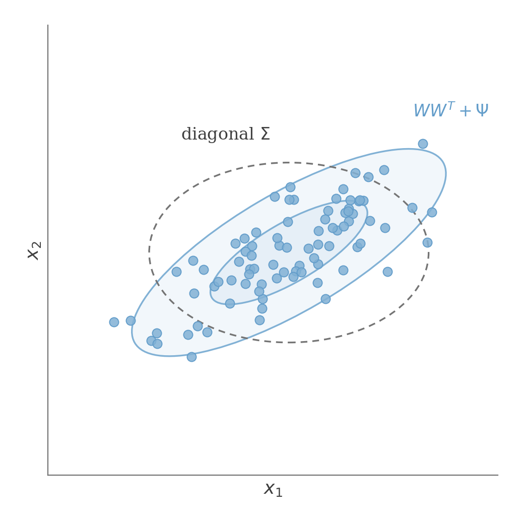
Factor analysis keeps the model compact while still allowing correlations by using a lower-dimensional latent variable.
Let:
x ∈ R d
x\in\mathbb R^d
x ∈ R d and let:
z ∈ R k , k < d
z\in\mathbb R^k,
\qquad
k<d
z ∈ R k , k < d be a lower-dimensional latent variable.
The loading matrix is:
W ∈ R d × k
W\in\mathbb R^{d\times k}
W ∈ R d × k and:
Ψ ∈ R d × d
\Psi\in\mathbb R^{d\times d}
Ψ ∈ R d × d is a positive diagonal matrix.
The factor analysis model is:
z ∼ N ( 0 , I k )
z
\sim
\mathcal N(0,I_k)
z ∼ N ( 0 , I k ) x ∣ z ∼ N ( μ + W z , Ψ )
x\mid z
\sim
\mathcal N(\mu+Wz,\Psi)
x ∣ z ∼ N ( μ + W z , Ψ ) We can equivalently write:
z ∼ N ( 0 , I k )
z
\sim
\mathcal N(0,I_k)
z ∼ N ( 0 , I k ) ϵ ∼ N ( 0 , Ψ )
\epsilon
\sim
\mathcal N(0,\Psi)
ϵ ∼ N ( 0 , Ψ ) x = μ + W z + ϵ
x
=
\mu+Wz+\epsilon
x = μ + W z + ϵ We assume z z z ϵ \epsilon ϵ
The latent variable z z z ϵ \epsilon ϵ
For a random variable:
x ∼ N ( μ , σ 2 )
x
\sim
\mathcal N(\mu,\sigma^2)
x ∼ N ( μ , σ 2 ) we can write:
x = μ + σ ϵ
x
=
\mu+\sigma\epsilon
x = μ + σ ϵ where:
ϵ ∼ N ( 0 , 1 )
\epsilon
\sim
\mathcal N(0,1)
ϵ ∼ N ( 0 , 1 ) Because x x x
Its distribution is:
x ∼ N ( μ , W W T + Ψ )
x
\sim
\mathcal N
\left(
\mu,
WW^T+\Psi
\right)
x ∼ N ( μ , W W T + Ψ ) A diagonal Σ \Sigma Σ W W T + Ψ WW^T+\Psi W W T + Ψ
The loading matrix is not unique.
For any orthogonal matrix:
R ∈ R k × k
R\in\mathbb R^{k\times k}
R ∈ R k × k replacing W W W W R WR W R z z z R T z R^Tz R T z
W W T + Ψ
WW^T+\Psi
W W T + Ψ This creates a rotational ambiguity, so the orientation of the latent factors is not uniquely identified.
More generally, because Ψ \Psi Ψ
› See derivationE [ x ] = E [ μ + W z + ϵ ]
\mathbb E[x]
=
\mathbb E[\mu+Wz+\epsilon]
E [ x ] = E [ μ + W z + ϵ ] = E [ μ ] + E [ W z ] + E [ ϵ ]
=
\mathbb E[\mu]
+
\mathbb E[Wz]
+
\mathbb E[\epsilon]
= E [ μ ] + E [ W z ] + E [ ϵ ] = μ + W E [ z ] + E [ ϵ ]
=
\mu
+
W\mathbb E[z]
+
\mathbb E[\epsilon]
= μ + W E [ z ] + E [ ϵ ] i Expectation is linear, and μ \mu μ W W W
i Both z z z ϵ \epsilon ϵ 0 0 0
Now consider the covariance:
Var ( x ) = E [ ( x − E [ x ] ) ( x − E [ x ] ) T ]
\operatorname{Var}(x)
=
\mathbb E
\left[
(x-\mathbb E[x])
(x-\mathbb E[x])^T
\right]
Var ( x ) = E [ ( x − E [ x ]) ( x − E [ x ] ) T ] = E [ ( μ + W z + ϵ − μ ) ( μ + W z + ϵ − μ ) T ]
=
\mathbb E
\left[
(\mu+Wz+\epsilon-\mu)
(\mu+Wz+\epsilon-\mu)^T
\right]
= E [ ( μ + W z + ϵ − μ ) ( μ + W z + ϵ − μ ) T ] = E [ ( W z + ϵ ) ( W z + ϵ ) T ]
=
\mathbb E
\left[
(Wz+\epsilon)
(Wz+\epsilon)^T
\right]
= E [ ( W z + ϵ ) ( W z + ϵ ) T ] = E [ W z z T W T + W z ϵ T + ϵ z T W T + ϵ ϵ T ]
=
\mathbb E
\left[
Wzz^TW^T
+
Wz\epsilon^T
+
\epsilon z^TW^T
+
\epsilon\epsilon^T
\right]
= E [ W z z T W T + W z ϵ T + ϵ z T W T + ϵ ϵ T ] = W E [ z z T ] W T + W E [ z ϵ T ] + E [ ϵ z T ] W T + E [ ϵ ϵ T ]
=
W\mathbb E[zz^T]W^T
+
W\mathbb E[z\epsilon^T]
+
\mathbb E[\epsilon z^T]W^T
+
\mathbb E[\epsilon\epsilon^T]
= W E [ z z T ] W T + W E [ z ϵ T ] + E [ ϵ z T ] W T + E [ ϵ ϵ T ] = W E [ z z T ] W T + E [ ϵ ϵ T ]
=
W\mathbb E[zz^T]W^T
+
\mathbb E[\epsilon\epsilon^T]
= W E [ z z T ] W T + E [ ϵ ϵ T ] i Because z z z ϵ \epsilon ϵ 0 0 0
= W W T + Ψ
=
WW^T+\Psi
= W W T + Ψ i Since E [ z z T ] = I k \mathbb E[zz^T]=I_k E [ z z T ] = I k E [ ϵ ϵ T ] = Ψ \mathbb E[\epsilon\epsilon^T]=\Psi E [ ϵ ϵ T ] = Ψ
Thus, the log-likelihood of the data under the model is:
ℓ ( μ , W , Ψ ) = log ∏ i = 1 n 1 ( 2 π ) d / 2 ∣ W W T + Ψ ∣ 1 / 2 exp ( − 1 2 ( x ( i ) − μ ) T ( W W T + Ψ ) − 1 ( x ( i ) − μ ) )
\ell(\mu,W,\Psi)
=
\log
\prod_{i=1}^{n}
\frac{
1
}{
(2\pi)^{d/2}
|WW^T+\Psi|^{1/2}
}
\exp
\left(
-\frac12
(x^{(i)}-\mu)^T
(WW^T+\Psi)^{-1}
(x^{(i)}-\mu)
\right)
ℓ ( μ , W , Ψ ) = log i = 1 ∏ n ( 2 π ) d /2 ∣ W W T + Ψ ∣ 1/2 1 exp ( − 2 1 ( x ( i ) − μ ) T ( W W T + Ψ ) − 1 ( x ( i ) − μ ) ) The mean has the closed-form estimate:
μ = 1 n ∑ i = 1 n x ( i )
\mu
=
\frac1n
\sum_{i=1}^n
x^{(i)}
μ = n 1 i = 1 ∑ n x ( i ) The parameters W W W Ψ \Psi Ψ
W W T + Ψ
WW^T+\Psi
W W T + Ψ so we estimate them using Expectation Maximization .
Posterior Inference
In the E-step, we infer the latent factors z z z W W W Ψ \Psi Ψ
Because the model is linear-Gaussian, the posterior p ( z ∣ x ) p(z\mid x) p ( z ∣ x )
z ∣ x ∼ N ( μ z ∣ x , Σ z ∣ x )
z\mid x
\sim
\mathcal N
\left(
\mu_{z\mid x},
\Sigma_{z\mid x}
\right)
z ∣ x ∼ N ( μ z ∣ x , Σ z ∣ x ) where:
μ z ∣ x = W T ( W W T + Ψ ) − 1 ( x − μ )
\mu_{z\mid x}
=
W^T
\left(
WW^T+\Psi
\right)^{-1}
(x-\mu)
μ z ∣ x = W T ( W W T + Ψ ) − 1 ( x − μ ) and:
Σ z ∣ x = I k − W T ( W W T + Ψ ) − 1 W
\Sigma_{z\mid x}
=
I_k
-
W^T
\left(
WW^T+\Psi
\right)^{-1}
W
Σ z ∣ x = I k − W T ( W W T + Ψ ) − 1 W For fixed model parameters, every observation has the same posterior covariance, but a different posterior mean determined by x − μ x-\mu x − μ
› See derivationFor jointly Gaussian random vectors z z z x x x z ∣ x z\mid x z ∣ x
z ∣ x ∼ N ( μ z ∣ x , Σ z ∣ x )
z\mid x
\sim
\mathcal N
\left(
\mu_{z\mid x},
\Sigma_{z\mid x}
\right)
z ∣ x ∼ N ( μ z ∣ x , Σ z ∣ x ) with:
μ z ∣ x = μ z + Σ z x Σ x x − 1 ( x − μ x )
\mu_{z\mid x}
=
\mu_z
+
\Sigma_{zx}
\Sigma_{xx}^{-1}
(x-\mu_x)
μ z ∣ x = μ z + Σ z x Σ xx − 1 ( x − μ x ) and:
Σ z ∣ x = Σ z z − Σ z x Σ x x − 1 Σ x z
\Sigma_{z\mid x}
=
\Sigma_{zz}
-
\Sigma_{zx}
\Sigma_{xx}^{-1}
\Sigma_{xz}
Σ z ∣ x = Σ zz − Σ z x Σ xx − 1 Σ x z From the model:
μ z = 0
\mu_z=0
μ z = 0 and:
Σ z z = Var ( z ) = I k
\Sigma_{zz}
=
\operatorname{Var}(z)
=
I_k
Σ zz = Var ( z ) = I k From the marginal distribution of x x x
μ x = μ
\mu_x=\mu
μ x = μ and:
Σ x x = W W T + Ψ
\Sigma_{xx}
=
WW^T+\Psi
Σ xx = W W T + Ψ Now:
Σ z x = Cov ( z , x )
\Sigma_{zx}
=
\operatorname{Cov}(z,x)
Σ z x = Cov ( z , x ) = E [ ( z − E [ z ] ) ( x − E [ x ] ) T ]
=
\mathbb E
\left[
(z-\mathbb E[z])
(x-\mathbb E[x])^T
\right]
= E [ ( z − E [ z ]) ( x − E [ x ] ) T ] = E [ z ( x − μ ) T ]
=
\mathbb E
\left[
z(x-\mu)^T
\right]
= E [ z ( x − μ ) T ] i Since E [ z ] = 0 \mathbb E[z]=0 E [ z ] = 0 E [ x ] = μ \mathbb E[x]=\mu E [ x ] = μ
= E [ z ( W z + ϵ ) T ]
=
\mathbb E
\left[
z(Wz+\epsilon)^T
\right]
= E [ z ( W z + ϵ ) T ] i Using x = μ + W z + ϵ x=\mu+Wz+\epsilon x = μ + W z + ϵ
= E [ z z T W T ] + E [ z ϵ T ]
=
\mathbb E
\left[
zz^TW^T
\right]
+
\mathbb E
\left[
z\epsilon^T
\right]
= E [ z z T W T ] + E [ z ϵ T ] = E [ z z T ] W T
=
\mathbb E[zz^T]W^T
= E [ z z T ] W T i Because z z z ϵ \epsilon ϵ 0 0 0 E [ z ϵ T ] = 0 \mathbb E[z\epsilon^T]=0 E [ z ϵ T ] = 0
i Since E [ z z T ] = I k \mathbb E[zz^T]=I_k E [ z z T ] = I k
Similarly:
Σ x z = Cov ( x , z ) = W
\Sigma_{xz}
=
\operatorname{Cov}(x,z)
=
W
Σ x z = Cov ( x , z ) = W Putting everything together:
z ∣ x ∼ N ( μ z ∣ x , Σ z ∣ x )
z\mid x
\sim
\mathcal N
\left(
\mu_{z\mid x},
\Sigma_{z\mid x}
\right)
z ∣ x ∼ N ( μ z ∣ x , Σ z ∣ x ) with:
μ z ∣ x = W T ( W W T + Ψ ) − 1 ( x − μ )
\mu_{z\mid x}
=
W^T
\left(
WW^T+\Psi
\right)^{-1}
(x-\mu)
μ z ∣ x = W T ( W W T + Ψ ) − 1 ( x − μ ) and:
Σ z ∣ x = I k − W T ( W W T + Ψ ) − 1 W
\Sigma_{z\mid x}
=
I_k
-
W^T
\left(
WW^T+\Psi
\right)^{-1}
W
Σ z ∣ x = I k − W T ( W W T + Ψ ) − 1 W The E-step for EM is therefore:
Q i ( z ( i ) ) = p ( z ( i ) ∣ x ( i ) ; μ , W , Ψ )
Q_i(z^{(i)})
=
p
\left(
z^{(i)}
\mid
x^{(i)};
\mu,W,\Psi
\right)
Q i ( z ( i ) ) = p ( z ( i ) ∣ x ( i ) ; μ , W , Ψ ) = 1 ( 2 π ) k / 2 ∣ Σ z ( i ) ∣ x ( i ) ∣ 1 / 2 exp ( − 1 2 ( z ( i ) − μ z ( i ) ∣ x ( i ) ) T Σ z ( i ) ∣ x ( i ) − 1 ( z ( i ) − μ z ( i ) ∣ x ( i ) ) )
=
\frac{
1
}{
(2\pi)^{k/2}
|\Sigma_{z^{(i)}\mid x^{(i)}}|^{1/2}
}
\exp
\left(
-\frac12
\left(
z^{(i)}-\mu_{z^{(i)}\mid x^{(i)}}
\right)^T
\Sigma_{z^{(i)}\mid x^{(i)}}^{-1}
\left(
z^{(i)}-\mu_{z^{(i)}\mid x^{(i)}}
\right)
\right)
= ( 2 π ) k /2 ∣ Σ z ( i ) ∣ x ( i ) ∣ 1/2 1 exp ( − 2 1 ( z ( i ) − μ z ( i ) ∣ x ( i ) ) T Σ z ( i ) ∣ x ( i ) − 1 ( z ( i ) − μ z ( i ) ∣ x ( i ) ) ) EM Parameter Updates
In the M-step, we maximize the evidence lower bound:
L ( D ; Q , μ , W , Ψ ) = ∑ i = 1 n E z ( i ) ∼ Q i [ log p ( x ( i ) , z ( i ) ; μ , W , Ψ ) Q i ( z ( i ) ) ]
\mathcal L
\left(
\mathcal D;
Q,
\mu,
W,
\Psi
\right)
=
\sum_{i=1}^n
\mathbb E_{z^{(i)}\sim Q_i}
\left[
\log
\frac{
p(x^{(i)},z^{(i)};\mu,W,\Psi)
}{
Q_i(z^{(i)})
}
\right]
L ( D ; Q , μ , W , Ψ ) = i = 1 ∑ n E z ( i ) ∼ Q i [ log Q i ( z ( i ) ) p ( x ( i ) , z ( i ) ; μ , W , Ψ ) ] The marginal model has mean μ \mu μ
We calculate this once and center the data before running EM:
μ = 1 n ∑ i = 1 n x ( i )
\mu
=
\frac1n
\sum_{i=1}^n
x^{(i)}
μ = n 1 i = 1 ∑ n x ( i ) The M-step only needs the first two moments of each posterior Q i Q_i Q i
m i = E Q i [ z ( i ) ] = μ z ( i ) ∣ x ( i )
m_i
=
\mathbb E_{Q_i}[z^{(i)}]
=
\mu_{z^{(i)}\mid x^{(i)}}
m i = E Q i [ z ( i ) ] = μ z ( i ) ∣ x ( i ) and:
C i = E Q i [ z ( i ) z ( i ) T ]
C_i
=
\mathbb E_{Q_i}
\left[
z^{(i)}z^{(i)T}
\right]
C i = E Q i [ z ( i ) z ( i ) T ] = Σ z ( i ) ∣ x ( i ) + m i m i T
=
\Sigma_{z^{(i)}\mid x^{(i)}}
+
m_im_i^T
= Σ z ( i ) ∣ x ( i ) + m i m i T At EM iteration t t t m i m_i m i C i C_i C i
( W ( t ) , Ψ ( t ) )
(W^{(t)},\Psi^{(t)})
( W ( t ) , Ψ ( t ) ) These moments remain fixed throughout the M-step.
The remaining updates are:
W = ( ∑ i = 1 n ( x ( i ) − μ ) m i T ) ( ∑ i = 1 n C i ) − 1
W
=
\left(
\sum_{i=1}^n
(x^{(i)}-\mu)m_i^T
\right)
\left(
\sum_{i=1}^n
C_i
\right)^{-1}
W = ( i = 1 ∑ n ( x ( i ) − μ ) m i T ) ( i = 1 ∑ n C i ) − 1 and:
Ψ = diag ( 1 n ∑ i = 1 n E Q i [ ( x ( i ) − μ − W z ( i ) ) ( x ( i ) − μ − W z ( i ) ) T ] )
\Psi
=
\operatorname{diag}
\left(
\frac1n
\sum_{i=1}^n
\mathbb E_{Q_i}
\left[
(x^{(i)}-\mu-Wz^{(i)})
(x^{(i)}-\mu-Wz^{(i)})^T
\right]
\right)
Ψ = diag ( n 1 i = 1 ∑ n E Q i [ ( x ( i ) − μ − W z ( i ) ) ( x ( i ) − μ − W z ( i ) ) T ] ) Intuitively, W W W Ψ \Psi Ψ
› See derivationL ( D ; Q , μ , W , Ψ ) = ∑ i = 1 n E z ( i ) ∼ Q i [ log p ( x ( i ) , z ( i ) ; μ , W , Ψ ) Q i ( z ( i ) ) ]
\mathcal L
\left(
\mathcal D;
Q,
\mu,
W,
\Psi
\right)
=
\sum_{i=1}^n
\mathbb E_{z^{(i)}\sim Q_i}
\left[
\log
\frac{
p(x^{(i)},z^{(i)};\mu,W,\Psi)
}{
Q_i(z^{(i)})
}
\right]
L ( D ; Q , μ , W , Ψ ) = i = 1 ∑ n E z ( i ) ∼ Q i [ log Q i ( z ( i ) ) p ( x ( i ) , z ( i ) ; μ , W , Ψ ) ] = ∑ i = 1 n E z ( i ) ∼ Q i [ log p ( x ( i ) ∣ z ( i ) ; μ , W , Ψ ) + log p ( z ( i ) ) − log Q i ( z ( i ) ) ]
=
\sum_{i=1}^n
\mathbb E_{z^{(i)}\sim Q_i}
\left[
\log
p(x^{(i)}\mid z^{(i)};\mu,W,\Psi)
+
\log p(z^{(i)})
-
\log Q_i(z^{(i)})
\right]
= i = 1 ∑ n E z ( i ) ∼ Q i [ log p ( x ( i ) ∣ z ( i ) ; μ , W , Ψ ) + log p ( z ( i ) ) − log Q i ( z ( i ) ) ] J ( μ , W , Ψ ) = ∑ i = 1 n E z ( i ) ∼ Q i [ log p ( x ( i ) ∣ z ( i ) ; μ , W , Ψ ) ]
\mathcal J(\mu,W,\Psi)
=
\sum_{i=1}^n
\mathbb E_{z^{(i)}\sim Q_i}
\left[
\log
p(x^{(i)}\mid z^{(i)};\mu,W,\Psi)
\right]
J ( μ , W , Ψ ) = i = 1 ∑ n E z ( i ) ∼ Q i [ log p ( x ( i ) ∣ z ( i ) ; μ , W , Ψ ) ] i During the M-step, Q i Q_i Q i p ( z ( i ) ) p(z^{(i)}) p ( z ( i ) ) Q i ( z ( i ) ) Q_i(z^{(i)}) Q i ( z ( i ) ) μ \mu μ W W W Ψ \Psi Ψ
Therefore:
J ( μ , W , Ψ ) = ∑ i = 1 n E z ( i ) ∼ Q i [ log ( 1 ( 2 π ) d / 2 ∣ Ψ ∣ 1 / 2 exp ( − 1 2 ( x ( i ) − μ − W z ( i ) ) T Ψ − 1 ( x ( i ) − μ − W z ( i ) ) ) ) ]
\mathcal J(\mu,W,\Psi)
=
\sum_{i=1}^{n}
\mathbb E_{z^{(i)}\sim Q_i}
\left[
\log
\left(
\frac{
1
}{
(2\pi)^{d/2}|\Psi|^{1/2}
}
\exp
\left(
-\frac12
(x^{(i)}-\mu-Wz^{(i)})^T
\Psi^{-1}
(x^{(i)}-\mu-Wz^{(i)})
\right)
\right)
\right]
J ( μ , W , Ψ ) = i = 1 ∑ n E z ( i ) ∼ Q i [ log ( ( 2 π ) d /2 ∣Ψ ∣ 1/2 1 exp ( − 2 1 ( x ( i ) − μ − W z ( i ) ) T Ψ − 1 ( x ( i ) − μ − W z ( i ) ) ) ) ] = ∑ i = 1 n E z ( i ) ∼ Q i [ − 1 2 log ∣ Ψ ∣ − d 2 log ( 2 π ) − 1 2 ( x ( i ) − μ − W z ( i ) ) T Ψ − 1 ( x ( i ) − μ − W z ( i ) ) ]
=
\sum_{i=1}^{n}
\mathbb E_{z^{(i)}\sim Q_i}
\left[
-\frac12\log|\Psi|
-
\frac d2\log(2\pi)
-
\frac12
(x^{(i)}-\mu-Wz^{(i)})^T
\Psi^{-1}
(x^{(i)}-\mu-Wz^{(i)})
\right]
= i = 1 ∑ n E z ( i ) ∼ Q i [ − 2 1 log ∣Ψ∣ − 2 d log ( 2 π ) − 2 1 ( x ( i ) − μ − W z ( i ) ) T Ψ − 1 ( x ( i ) − μ − W z ( i ) ) ] The marginal distribution is:
x ∼ N ( μ , W W T + Ψ )
x
\sim
\mathcal N
\left(
\mu,
WW^T+\Psi
\right)
x ∼ N ( μ , W W T + Ψ ) For any fixed covariance, differentiating its observed-data log-likelihood with respect to μ \mu μ
μ = 1 n ∑ i = 1 n x ( i )
\mu
=
\frac1n
\sum_{i=1}^n
x^{(i)}
μ = n 1 i = 1 ∑ n x ( i ) We therefore calculate μ \mu μ
With centered data, each posterior mean is a linear transformation of x ( i ) − μ x^{(i)}-\mu x ( i ) − μ
∑ i m i = 0
\sum_i m_i=0
i ∑ m i = 0 exactly.
For matrices of compatible dimensions:
∇ A tr ( A B A T C ) = C A B + C T A B T
\nabla_A
\operatorname{tr}
\left(
ABA^TC
\right)
=
CAB
+
C^TAB^T
∇ A tr ( A B A T C ) = C A B + C T A B T Taking the derivative with respect to W W W
− 1 2 ∇ W ∑ i = 1 n E z ( i ) ∼ Q i [ ( x ( i ) − μ − W z ( i ) ) T Ψ − 1 ( x ( i ) − μ − W z ( i ) ) ]
-\frac12
\nabla_W
\sum_{i=1}^{n}
\mathbb E_{z^{(i)}\sim Q_i}
\left[
(x^{(i)}-\mu-Wz^{(i)})^T
\Psi^{-1}
(x^{(i)}-\mu-Wz^{(i)})
\right]
− 2 1 ∇ W i = 1 ∑ n E z ( i ) ∼ Q i [ ( x ( i ) − μ − W z ( i ) ) T Ψ − 1 ( x ( i ) − μ − W z ( i ) ) ] = − 1 2 ∑ i = 1 n E z ( i ) ∼ Q i [ − ∇ W ( z ( i ) T W T Ψ − 1 ( x ( i ) − μ ) )
=
-\frac12
\sum_{i=1}^{n}
\mathbb E_{z^{(i)}\sim Q_i}
\left[
-\nabla_W
\left(
z^{(i)T}
W^T
\Psi^{-1}
(x^{(i)}-\mu)
\right)
\right. = − 2 1 i = 1 ∑ n E z ( i ) ∼ Q i [ − ∇ W ( z ( i ) T W T Ψ − 1 ( x ( i ) − μ ) ) i + ∇ W ( z ( i ) T W T Ψ − 1 W z ( i ) ) − ∇ W ( ( x ( i ) − μ ) T Ψ − 1 W z ( i ) ) ]
\left.
+
\nabla_W
\left(
z^{(i)T}
W^T
\Psi^{-1}
W
z^{(i)}
\right)
-
\nabla_W
\left(
(x^{(i)}-\mu)^T
\Psi^{-1}
Wz^{(i)}
\right)
\right]
+ ∇ W ( z ( i ) T W T Ψ − 1 W z ( i ) ) − ∇ W ( ( x ( i ) − μ ) T Ψ − 1 W z ( i ) ) ] Terms that do not depend on W W W 0 0 0
= − 1 2 ∑ i = 1 n E z ( i ) ∼ Q i [ − ∇ W tr ( z ( i ) T W T Ψ − 1 ( x ( i ) − μ ) )
=
-\frac12
\sum_{i=1}^{n}
\mathbb E_{z^{(i)}\sim Q_i}
\left[
-\nabla_W
\operatorname{tr}
\left(
z^{(i)T}
W^T
\Psi^{-1}
(x^{(i)}-\mu)
\right)
\right. = − 2 1 i = 1 ∑ n E z ( i ) ∼ Q i [ − ∇ W tr ( z ( i ) T W T Ψ − 1 ( x ( i ) − μ ) ) i + ∇ W tr ( z ( i ) T W T Ψ − 1 W z ( i ) ) − ∇ W tr ( ( x ( i ) − μ ) T Ψ − 1 W z ( i ) ) ]
\left.
+
\nabla_W
\operatorname{tr}
\left(
z^{(i)T}
W^T
\Psi^{-1}
Wz^{(i)}
\right)
-
\nabla_W
\operatorname{tr}
\left(
(x^{(i)}-\mu)^T
\Psi^{-1}
Wz^{(i)}
\right)
\right]
+ ∇ W tr ( z ( i ) T W T Ψ − 1 W z ( i ) ) − ∇ W tr ( ( x ( i ) − μ ) T Ψ − 1 W z ( i ) ) ] Each term is a scalar, and a scalar is equal to its trace.
= − 1 2 ∑ i = 1 n E z ( i ) ∼ Q i [ − ∇ W tr ( z ( i ) T W T Ψ − 1 ( x ( i ) − μ ) )
=
-\frac12
\sum_{i=1}^{n}
\mathbb E_{z^{(i)}\sim Q_i}
\left[
-\nabla_W
\operatorname{tr}
\left(
z^{(i)T}
W^T
\Psi^{-1}
(x^{(i)}-\mu)
\right)
\right. = − 2 1 i = 1 ∑ n E z ( i ) ∼ Q i [ − ∇ W tr ( z ( i ) T W T Ψ − 1 ( x ( i ) − μ ) ) i + ∇ W tr ( z ( i ) T W T Ψ − 1 W z ( i ) ) − ∇ W tr ( z ( i ) T W T Ψ − T ( x ( i ) − μ ) ) ]
\left.
+
\nabla_W
\operatorname{tr}
\left(
z^{(i)T}
W^T
\Psi^{-1}
Wz^{(i)}
\right)
-
\nabla_W
\operatorname{tr}
\left(
z^{(i)T}
W^T
\Psi^{-T}
(x^{(i)}-\mu)
\right)
\right]
+ ∇ W tr ( z ( i ) T W T Ψ − 1 W z ( i ) ) − ∇ W tr ( z ( i ) T W T Ψ − T ( x ( i ) − μ ) ) ] Using tr ( A B ) = tr ( B A ) \operatorname{tr}(AB)=\operatorname{tr}(BA) tr ( A B ) = tr ( B A ) tr ( A T ) = tr ( A ) \operatorname{tr}(A^T)=\operatorname{tr}(A) tr ( A T ) = tr ( A )
= − 1 2 ∑ i = 1 n E z ( i ) ∼ Q i [ − 2 ∇ W tr ( z ( i ) T W T Ψ − 1 ( x ( i ) − μ ) )
=
-\frac12
\sum_{i=1}^{n}
\mathbb E_{z^{(i)}\sim Q_i}
\left[
-2
\nabla_W
\operatorname{tr}
\left(
z^{(i)T}
W^T
\Psi^{-1}
(x^{(i)}-\mu)
\right)
\right. = − 2 1 i = 1 ∑ n E z ( i ) ∼ Q i [ − 2 ∇ W tr ( z ( i ) T W T Ψ − 1 ( x ( i ) − μ ) ) i + ∇ W tr ( z ( i ) T W T Ψ − 1 W z ( i ) ) ]
\left.
+
\nabla_W
\operatorname{tr}
\left(
z^{(i)T}
W^T
\Psi^{-1}
Wz^{(i)}
\right)
\right]
+ ∇ W tr ( z ( i ) T W T Ψ − 1 W z ( i ) ) ] Since Ψ \Psi Ψ Ψ − T = Ψ − 1 \Psi^{-T}=\Psi^{-1} Ψ − T = Ψ − 1
= − 1 2 ∑ i = 1 n E z ( i ) ∼ Q i [ − 2 ∇ W tr ( W T Ψ − 1 ( x ( i ) − μ ) z ( i ) T )
=
-\frac12
\sum_{i=1}^{n}
\mathbb E_{z^{(i)}\sim Q_i}
\left[
-2
\nabla_W
\operatorname{tr}
\left(
W^T
\Psi^{-1}
(x^{(i)}-\mu)
z^{(i)T}
\right)
\right. = − 2 1 i = 1 ∑ n E z ( i ) ∼ Q i [ − 2 ∇ W tr ( W T Ψ − 1 ( x ( i ) − μ ) z ( i ) T ) i + ∇ W tr ( W z ( i ) z ( i ) T W T Ψ − 1 ) ]
\left.
+
\nabla_W
\operatorname{tr}
\left(
Wz^{(i)}z^{(i)T}W^T\Psi^{-1}
\right)
\right]
+ ∇ W tr ( W z ( i ) z ( i ) T W T Ψ − 1 ) ] Using cyclic permutation of the trace.
= − 1 2 ∑ i = 1 n E z ( i ) ∼ Q i [ − 2 Ψ − 1 ( x ( i ) − μ ) z ( i ) T + Ψ − 1 W z ( i ) z ( i ) T + Ψ − T W z ( i ) z ( i ) T ]
=
-\frac12
\sum_{i=1}^{n}
\mathbb E_{z^{(i)}\sim Q_i}
\left[
-2
\Psi^{-1}
(x^{(i)}-\mu)
z^{(i)T}
+
\Psi^{-1}
Wz^{(i)}z^{(i)T}
+
\Psi^{-T}
Wz^{(i)}z^{(i)T}
\right]
= − 2 1 i = 1 ∑ n E z ( i ) ∼ Q i [ − 2 Ψ − 1 ( x ( i ) − μ ) z ( i ) T + Ψ − 1 W z ( i ) z ( i ) T + Ψ − T W z ( i ) z ( i ) T ] i Using the matrix derivative identity above.
= ∑ i = 1 n E z ( i ) ∼ Q i [ Ψ − 1 ( x ( i ) − μ ) z ( i ) T − Ψ − 1 W z ( i ) z ( i ) T ]
=
\sum_{i=1}^{n}
\mathbb E_{z^{(i)}\sim Q_i}
\left[
\Psi^{-1}
(x^{(i)}-\mu)
z^{(i)T}
-
\Psi^{-1}
Wz^{(i)}z^{(i)T}
\right]
= i = 1 ∑ n E z ( i ) ∼ Q i [ Ψ − 1 ( x ( i ) − μ ) z ( i ) T − Ψ − 1 W z ( i ) z ( i ) T ] i Again using Ψ − T = Ψ − 1 \Psi^{-T}=\Psi^{-1} Ψ − T = Ψ − 1
Setting the derivative equal to 0 0 0
Ψ − 1 ( ∑ i = 1 n E Q i [ ( x ( i ) − μ ) z ( i ) T ] )
\Psi^{-1}
\left(
\sum_{i=1}^{n}
\mathbb E_{Q_i}
\left[
(x^{(i)}-\mu)z^{(i)T}
\right]
\right)
Ψ − 1 ( i = 1 ∑ n E Q i [ ( x ( i ) − μ ) z ( i ) T ] ) = Ψ − 1 W ( ∑ i = 1 n E Q i [ z ( i ) z ( i ) T ] )
=
\Psi^{-1}
W
\left(
\sum_{i=1}^{n}
\mathbb E_{Q_i}
\left[
z^{(i)}z^{(i)T}
\right]
\right)
= Ψ − 1 W ( i = 1 ∑ n E Q i [ z ( i ) z ( i ) T ] ) Therefore:
W = ( ∑ i = 1 n ( x ( i ) − μ ) E Q i [ z ( i ) T ] ) ( ∑ i = 1 n E Q i [ z ( i ) z ( i ) T ] ) − 1
W
=
\left(
\sum_{i=1}^{n}
(x^{(i)}-\mu)
\mathbb E_{Q_i}
[z^{(i)T}]
\right)
\left(
\sum_{i=1}^{n}
\mathbb E_{Q_i}
[z^{(i)}z^{(i)T}]
\right)^{-1}
W = ( i = 1 ∑ n ( x ( i ) − μ ) E Q i [ z ( i ) T ] ) ( i = 1 ∑ n E Q i [ z ( i ) z ( i ) T ] ) − 1 = ( ∑ i = 1 n ( x ( i ) − μ ) m i T ) ( ∑ i = 1 n ( m i m i T + Σ z ( i ) ∣ x ( i ) ) ) − 1
=
\left(
\sum_{i=1}^{n}
(x^{(i)}-\mu)m_i^T
\right)
\left(
\sum_{i=1}^{n}
\left(
m_im_i^T
+
\Sigma_{z^{(i)}\mid x^{(i)}}
\right)
\right)^{-1}
= ( i = 1 ∑ n ( x ( i ) − μ ) m i T ) ( i = 1 ∑ n ( m i m i T + Σ z ( i ) ∣ x ( i ) ) ) − 1 i Using E [ z z T ] = E [ z ] E [ z ] T + Cov ( z ) \mathbb E[zz^T]=\mathbb E[z]\mathbb E[z]^T+\operatorname{Cov}(z) E [ z z T ] = E [ z ] E [ z ] T + Cov ( z )
Thus:
W = ( ∑ i = 1 n ( x ( i ) − μ ) m i T ) ( ∑ i = 1 n C i ) − 1
W
=
\left(
\sum_{i=1}^{n}
(x^{(i)}-\mu)m_i^T
\right)
\left(
\sum_{i=1}^{n}
C_i
\right)^{-1}
W = ( i = 1 ∑ n ( x ( i ) − μ ) m i T ) ( i = 1 ∑ n C i ) − 1 For the diagonal-noise update, let:
r ( i ) = x ( i ) − μ − W z ( i )
r^{(i)}
=
x^{(i)}-\mu-Wz^{(i)}
r ( i ) = x ( i ) − μ − W z ( i ) and write:
Ψ = diag ( ψ 1 , … , ψ d )
\Psi
=
\operatorname{diag}
(\psi_1,\ldots,\psi_d)
Ψ = diag ( ψ 1 , … , ψ d ) The terms involving one diagonal entry ψ j \psi_j ψ j
− n 2 log ψ j − 1 2 ψ j ∑ i = 1 n E Q i [ ( r j ( i ) ) 2 ]
-\frac n2
\log\psi_j
-
\frac{1}{2\psi_j}
\sum_{i=1}^n
\mathbb E_{Q_i}
\left[
(r_j^{(i)})^2
\right]
− 2 n log ψ j − 2 ψ j 1 i = 1 ∑ n E Q i [ ( r j ( i ) ) 2 ] Setting the derivative with respect to ψ j \psi_j ψ j 0 0 0
ψ j = 1 n ∑ i = 1 n E Q i [ ( r j ( i ) ) 2 ]
\psi_j
=
\frac1n
\sum_{i=1}^n
\mathbb E_{Q_i}
\left[
(r_j^{(i)})^2
\right]
ψ j = n 1 i = 1 ∑ n E Q i [ ( r j ( i ) ) 2 ] Thus, if:
Φ = 1 n ∑ i = 1 n [ ( x ( i ) − μ ) ( x ( i ) − μ ) T − W m i ( x ( i ) − μ ) T
\Phi
=
\frac1n
\sum_{i=1}^n
\left[
(x^{(i)}-\mu)
(x^{(i)}-\mu)^T
-
Wm_i
(x^{(i)}-\mu)^T
\right. Φ = n 1 i = 1 ∑ n [ ( x ( i ) − μ ) ( x ( i ) − μ ) T − W m i ( x ( i ) − μ ) T − ( x ( i ) − μ ) m i T W T + W C i W T ]
\left.
-
(x^{(i)}-\mu)
m_i^TW^T
+
WC_iW^T
\right]
− ( x ( i ) − μ ) m i T W T + W C i W T ] then the constrained M-step is:
Ψ = diag ( Φ )
\Psi
=
\operatorname{diag}(\Phi)
Ψ = diag ( Φ ) Variational Autoencoders
Let:
z ∼ N ( 0 , I k )
z
\sim
\mathcal N(0,I_k)
z ∼ N ( 0 , I k ) be a latent variable, and let θ \theta θ
g ( z ; θ )
g(z;\theta)
g ( z ; θ ) that maps:
z ∈ R k
z\in\mathbb R^k
z ∈ R k to:
R d
\mathbb R^d
R d For real-valued observations, suppose the decoder likelihood is:
x ∣ z ∼ N ( g ( z ; θ ) , σ 2 I d )
x\mid z
\sim
\mathcal N
\left(
g(z;\theta),
\sigma^2I_d
\right)
x ∣ z ∼ N ( g ( z ; θ ) , σ 2 I d ) So the decoder takes a low-dimensional latent vector z z z x x x
Variational Inference and the VAE Objective
To train the model, we would ideally compute the posterior:
p ( z ∣ x ; θ )
p(z\mid x;\theta)
p ( z ∣ x ; θ ) In simple latent-variable models such as factor analysis, this posterior has a closed form.
With a nonlinear decoder g ( z ; θ ) g(z;\theta) g ( z ; θ )
p ( x ; θ ) = ∫ p ( x ∣ z ; θ ) p ( z ) d z
p(x;\theta)
=
\int
p(x\mid z;\theta)
p(z)\,dz
p ( x ; θ ) = ∫ p ( x ∣ z ; θ ) p ( z ) d z VAEs therefore approximate the posterior with a tractable distribution:
Q ( z ∣ x )
Q(z\mid x)
Q ( z ∣ x ) The ELBO would be tight if this approximate posterior were equal to the exact posterior.
Recall:
ELBO ( x ; Q , θ ) = log p ( x ; θ ) − D K L ( Q ( z ) ∥ p ( z ∣ x ; θ ) )
\text{ELBO}(x;Q,\theta)
=
\log p(x;\theta)
-
D_{KL}
\left(
Q(z)
\parallel
p(z\mid x;\theta)
\right)
ELBO ( x ; Q , θ ) = log p ( x ; θ ) − D K L ( Q ( z ) ∥ p ( z ∣ x ; θ ) ) Therefore:
log p ( x ; θ ) = ELBO ( x ; Q , θ ) + D K L ( Q ( z ) ∥ p ( z ∣ x ; θ ) )
\log p(x;\theta)
=
\text{ELBO}(x;Q,\theta)
+
D_{KL}
\left(
Q(z)
\parallel
p(z\mid x;\theta)
\right)
log p ( x ; θ ) = ELBO ( x ; Q , θ ) + D K L ( Q ( z ) ∥ p ( z ∣ x ; θ ) ) For fixed θ \theta θ Q \mathcal Q Q
Q θ ∗ ( z ∣ x ) = arg max Q ∈ Q ELBO ( x ; Q , θ )
Q_\theta^*(z\mid x)
=
\arg\max_{Q\in\mathcal Q}
\text{ELBO}(x;Q,\theta)
Q θ ∗ ( z ∣ x ) = arg Q ∈ Q max ELBO ( x ; Q , θ ) = arg min Q ∈ Q D K L ( Q ( z ) ∥ p ( z ∣ x ; θ ) )
=
\arg\min_{Q\in\mathcal Q}
D_{KL}
\left(
Q(z)
\parallel
p(z\mid x;\theta)
\right)
= arg Q ∈ Q min D K L ( Q ( z ) ∥ p ( z ∣ x ; θ ) ) If the exact posterior belongs to Q \mathcal Q Q
Q θ ∗ = p ( z ∣ x ; θ )
Q_\theta^*
=
p(z\mid x;\theta)
Q θ ∗ = p ( z ∣ x ; θ ) Otherwise, Q θ ∗ Q_\theta^* Q θ ∗
A common choice is a diagonal Gaussian approximate posterior:
Q ( z ∣ x ) = ∏ j = 1 k Q j ( z j ∣ x )
Q(z\mid x)
=
\prod_{j=1}^k
Q^j(z_j\mid x)
Q ( z ∣ x ) = j = 1 ∏ k Q j ( z j ∣ x ) The diagonal covariance means the latent coordinates are independent under Q ( z ∣ x ) Q(z\mid x) Q ( z ∣ x )
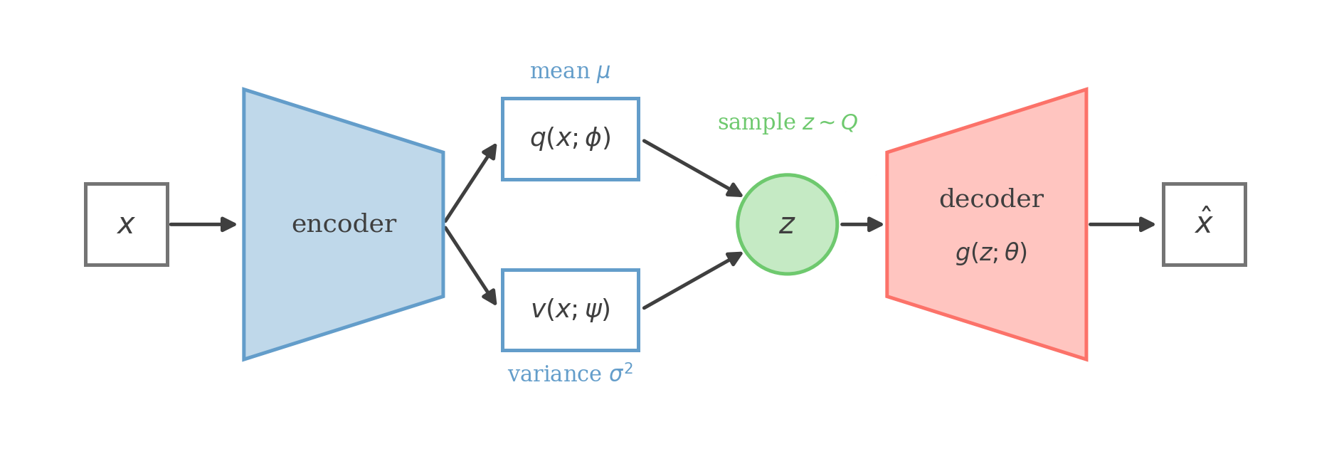
Let the encoder networks:
q ( x ; ϕ )
q(x;\phi)
q ( x ; ϕ ) and:
v ( x ; ψ )
v(x;\psi)
v ( x ; ψ ) output the posterior mean and a positive variance vector, respectively.
Then:
Q i ( z ( i ) ∣ x ( i ) ) = N ( q ( x ( i ) ; ϕ ) , diag ( v ( x ( i ) ; ψ ) ) )
Q_i
\left(
z^{(i)}
\mid
x^{(i)}
\right)
=
\mathcal N
\left(
q(x^{(i)};\phi),
\operatorname{diag}
\left(
v(x^{(i)};\psi)
\right)
\right)
Q i ( z ( i ) ∣ x ( i ) ) = N ( q ( x ( i ) ; ϕ ) , diag ( v ( x ( i ) ; ψ ) ) ) The encoder turns x x x Q Q Q q ( x ; ϕ ) q(x;\phi) q ( x ; ϕ ) v ( x ; ψ ) v(x;\psi) v ( x ; ψ ) z ∼ Q z\sim Q z ∼ Q x x x
The per-example ELBO is:
L i ( ϕ , ψ , θ ) = E z ∼ Q i [ log p ( x ( i ) ∣ z ; θ ) ] − D K L ( Q i ( z ∣ x ( i ) ) ∥ p ( z ) )
\mathcal L_i(\phi,\psi,\theta)
=
\mathbb E_{z\sim Q_i}
\left[
\log
p(x^{(i)}\mid z;\theta)
\right]
-
D_{KL}
\left(
Q_i(z\mid x^{(i)})
\parallel
p(z)
\right)
L i ( ϕ , ψ , θ ) = E z ∼ Q i [ log p ( x ( i ) ∣ z ; θ ) ] − D K L ( Q i ( z ∣ x ( i ) ) ∥ p ( z ) ) The two terms play different roles.
The reconstruction term :
E z ∼ Q i [ log p ( x ( i ) ∣ z ; θ ) ]
\mathbb E_{z\sim Q_i}
\left[
\log
p(x^{(i)}\mid z;\theta)
\right]
E z ∼ Q i [ log p ( x ( i ) ∣ z ; θ ) ] rewards latent samples that allow the decoder to explain x ( i ) x^{(i)} x ( i )
The KL term :
D K L ( Q i ( z ∣ x ( i ) ) ∥ p ( z ) )
D_{KL}
\left(
Q_i(z\mid x^{(i)})
\parallel
p(z)
\right)
D K L ( Q i ( z ∣ x ( i ) ) ∥ p ( z ) ) keeps the approximate posterior close to the prior.
With the fixed-variance Gaussian decoder:
log p ( x ∣ z ; θ ) = C − 1 2 σ 2 ∥ x − g ( z ; θ ) ∥ 2 2
\log p(x\mid z;\theta)
=
C
-
\frac{1}{2\sigma^2}
\left\|
x-g(z;\theta)
\right\|_2^2
log p ( x ∣ z ; θ ) = C − 2 σ 2 1 ∥ x − g ( z ; θ ) ∥ 2 2 where C C C θ \theta θ
Thus, maximizing the reconstruction term is equivalent to minimizing a scaled expected squared reconstruction error.
If the decoder variance is learned, its log-normalization term also matters, so the objective is not simply squared error.
The full-dataset objective is the sum of the per-example bounds:
L ( D ; ϕ , ψ , θ ) = ∑ i = 1 n L i ( ϕ , ψ , θ )
\mathcal L
\left(
\mathcal D;
\phi,
\psi,
\theta
\right)
=
\sum_{i=1}^n
\mathcal L_i
(\phi,\psi,\theta)
L ( D ; ϕ , ψ , θ ) = i = 1 ∑ n L i ( ϕ , ψ , θ ) Rather than computing separate variational parameters for every example, the encoder amortizes inference across the dataset.
We jointly optimize the encoder and decoder parameters using stochastic gradient ascent:
θ ← θ + η ∇ θ L ( D ; ϕ , ψ , θ )
\theta
\leftarrow
\theta
+
\eta
\nabla_\theta
\mathcal L
\left(
\mathcal D;
\phi,
\psi,
\theta
\right)
θ ← θ + η ∇ θ L ( D ; ϕ , ψ , θ ) ϕ ← ϕ + η ∇ ϕ L ( D ; ϕ , ψ , θ )
\phi
\leftarrow
\phi
+
\eta
\nabla_\phi
\mathcal L
\left(
\mathcal D;
\phi,
\psi,
\theta
\right)
ϕ ← ϕ + η ∇ ϕ L ( D ; ϕ , ψ , θ ) ψ ← ψ + η ∇ ψ L ( D ; ϕ , ψ , θ )
\psi
\leftarrow
\psi
+
\eta
\nabla_\psi
\mathcal L
\left(
\mathcal D;
\phi,
\psi,
\theta
\right)
ψ ← ψ + η ∇ ψ L ( D ; ϕ , ψ , θ ) The Reparameterization Trick
There is one remaining problem: the encoder parameters determine the distribution we sample z z z z z z
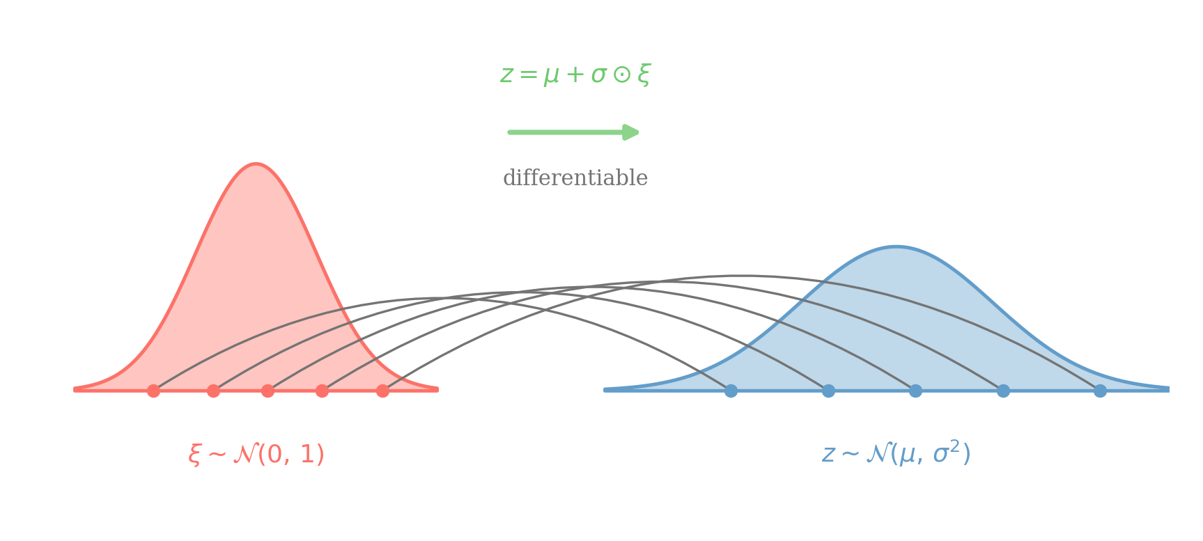
The reparameterization trick moves the randomness into a separate variable whose distribution does not depend on the encoder parameters.
Draw:
ξ ( i ) ∼ N ( 0 , I k )
\xi^{(i)}
\sim
\mathcal N(0,I_k)
ξ ( i ) ∼ N ( 0 , I k ) and define:
z ^ ( i ) = q ( x ( i ) ; ϕ ) + v ( x ( i ) ; ψ ) ⊙ ξ ( i )
\hat z^{(i)}
=
q(x^{(i)};\phi)
+
\sqrt{
v(x^{(i)};\psi)
}
\odot
\xi^{(i)}
z ^ ( i ) = q ( x ( i ) ; ϕ ) + v ( x ( i ) ; ψ ) ⊙ ξ ( i ) where the square root is applied elementwise.
Now the randomness is entirely in ξ ( i ) \xi^{(i)} ξ ( i ) z ^ ( i ) \hat z^{(i)} z ^ ( i )
Sampling z ∼ N ( μ , diag ( σ 2 ) ) z\sim\mathcal N(\mu,\operatorname{diag}(\sigma^2)) z ∼ N ( μ , diag ( σ 2 )) ξ ∼ N ( 0 , I k ) \xi\sim\mathcal N(0,I_k) ξ ∼ N ( 0 , I k ) z = μ + σ ⊙ ξ z=\mu+\sigma\odot\xi z = μ + σ ⊙ ξ σ = v \sigma=\sqrt v σ = v ξ \xi ξ
With this reparameterization, both the encoder and decoder can be trained using ordinary backpropagation.
The decoder gradient is:
∇ θ L ( D ) = ∑ i = 1 n E ξ ( i ) [ ∇ θ log p ( x ( i ) ∣ z ^ ( i ) ; θ ) ]
\nabla_\theta
\mathcal L(\mathcal D)
=
\sum_{i=1}^n
\mathbb E_{\xi^{(i)}}
\left[
\nabla_\theta
\log
p
\left(
x^{(i)}
\mid
\hat z^{(i)};
\theta
\right)
\right]
∇ θ L ( D ) = i = 1 ∑ n E ξ ( i ) [ ∇ θ log p ( x ( i ) ∣ z ^ ( i ) ; θ ) ] For either encoder parameter block:
η ∈ { ϕ , ψ }
\eta
\in
\{\phi,\psi\}
η ∈ { ϕ , ψ } we have:
∇ η L ( D ) = ∑ i = 1 n { E ξ ( i ) [ ∇ η log p ( x ( i ) ∣ z ^ ( i ) ; θ ) ] − ∇ η D K L ( Q i ( z ∣ x ( i ) ) ∥ p ( z ) ) }
\nabla_\eta
\mathcal L(\mathcal D)
=
\sum_{i=1}^n
\left\{
\mathbb E_{\xi^{(i)}}
\left[
\nabla_\eta
\log
p
\left(
x^{(i)}
\mid
\hat z^{(i)};
\theta
\right)
\right]
-
\nabla_\eta
D_{KL}
\left(
Q_i(z\mid x^{(i)})
\parallel
p(z)
\right)
\right\}
∇ η L ( D ) = i = 1 ∑ n { E ξ ( i ) [ ∇ η log p ( x ( i ) ∣ z ^ ( i ) ; θ ) ] − ∇ η D K L ( Q i ( z ∣ x ( i ) ) ∥ p ( z ) ) } These derivatives are computed by backpropagation.
We estimate each expectation using one or more Monte Carlo samples. A single latent sample per example is commonly used when training with minibatches.
› See derivationL ( D ) = ∑ i = 1 n { E z ∼ Q i [ log p ( x ( i ) ∣ z ; θ ) ] − D K L ( Q i ( z ∣ x ( i ) ) ∥ p ( z ) ) }
\mathcal L(\mathcal D)
=
\sum_{i=1}^n
\left\{
\mathbb E_{z\sim Q_i}
\left[
\log
p(x^{(i)}\mid z;\theta)
\right]
-
D_{KL}
\left(
Q_i(z\mid x^{(i)})
\parallel
p(z)
\right)
\right\}
L ( D ) = i = 1 ∑ n { E z ∼ Q i [ log p ( x ( i ) ∣ z ; θ ) ] − D K L ( Q i ( z ∣ x ( i ) ) ∥ p ( z ) ) } The reparameterization trick rewrites an expectation over the parameter-dependent distribution Q i Q_i Q i
E z ∼ Q i [ f ( z ) ] = E ξ ∼ N ( 0 , I k ) [ f ( q ( x ( i ) ; ϕ ) + v ( x ( i ) ; ψ ) ⊙ ξ ) ]
\mathbb E_{z\sim Q_i}
[f(z)]
=
\mathbb E_{
\xi\sim\mathcal N(0,I_k)
}
\left[
f
\left(
q(x^{(i)};\phi)
+
\sqrt{
v(x^{(i)};\psi)
}
\odot\xi
\right)
\right]
E z ∼ Q i [ f ( z )] = E ξ ∼ N ( 0 , I k ) [ f ( q ( x ( i ) ; ϕ ) + v ( x ( i ) ; ψ ) ⊙ ξ ) ] Under the usual differentiability and integrability conditions, for:
η ∈ { ϕ , ψ }
\eta\in\{\phi,\psi\}
η ∈ { ϕ , ψ } we can move the derivative inside this fixed-noise expectation:
∇ η E ξ [ f ( z ^ ( i ) ) ] = E ξ [ ∇ η f ( z ^ ( i ) ) ]
\nabla_\eta
\mathbb E_\xi
\left[
f(\hat z^{(i)})
\right]
=
\mathbb E_\xi
\left[
\nabla_\eta
f(\hat z^{(i)})
\right]
∇ η E ξ [ f ( z ^ ( i ) ) ] = E ξ [ ∇ η f ( z ^ ( i ) ) ] The decoder parameters θ \theta θ Q i Q_i Q i
Differentiating the same reparameterized term with respect to ϕ \phi ϕ ψ \psi ψ