Expectation Maximization
Suppose our model contains an observed variable x x x z z z
p ( x , z ; θ )
p(x,z;\theta)
p ( x , z ; θ ) To find the probability of the observed data x x x z z z
p ( x ; θ ) = ∑ z p ( x , z ; θ )
p(x;\theta)
=
\sum_z
p(x,z;\theta)
p ( x ; θ ) = z ∑ p ( x , z ; θ ) For a continuous latent variable, the sum is replaced by an integral:
p ( x ; θ ) = ∫ p ( x , z ; θ ) d z
p(x;\theta)
=
\int
p(x,z;\theta)\,dz
p ( x ; θ ) = ∫ p ( x , z ; θ ) d z We use sums below for notational simplicity.
For a dataset of n n n
ℓ ( θ ) = ∑ i = 1 n log p ( x ( i ) ; θ )
\ell(\theta)
=
\sum_{i=1}^n
\log p(x^{(i)};\theta)
ℓ ( θ ) = i = 1 ∑ n log p ( x ( i ) ; θ ) = ∑ i = 1 n log ∑ z ( i ) p ( x ( i ) , z ( i ) ; θ )
=
\sum_{i=1}^n
\log
\sum_{z^{(i)}}
p(x^{(i)},z^{(i)};\theta)
= i = 1 ∑ n log z ( i ) ∑ p ( x ( i ) , z ( i ) ; θ ) The difficulty is the sum over the latent variable inside the logarithm:
log ∑ z p ( x , z ; θ )
\log
\sum_z
p(x,z;\theta)
log z ∑ p ( x , z ; θ ) This often makes the likelihood difficult to optimize directly. EM handles this by constructing a lower bound on the log-likelihood and optimizing that bound instead.
The Evidence Lower Bound
To construct this lower bound, introduce a distribution Q ( z ) Q(z) Q ( z )
∑ z Q ( z ) = 1
\sum_z Q(z)=1
z ∑ Q ( z ) = 1 and Q ( z ) ≥ 0 Q(z)\geq0 Q ( z ) ≥ 0
We assume Q ( z ) > 0 Q(z)>0 Q ( z ) > 0 p ( x , z ; θ ) > 0 p(x,z;\theta)>0 p ( x , z ; θ ) > 0
Jensen's Inequality
Jensen's inequality states that for a convex function f f f
E [ f ( X ) ] ≥ f ( E [ X ] )
\mathbb{E}[f(X)]
\geq
f(\mathbb{E}[X])
E [ f ( X )] ≥ f ( E [ X ]) For a concave function, the inequality is reversed:
E [ f ( X ) ] ≤ f ( E [ X ] )
\mathbb{E}[f(X)]
\leq
f(\mathbb{E}[X])
E [ f ( X )] ≤ f ( E [ X ]) Also, if X X X
X = E [ X ]
X=\mathbb{E}[X]
X = E [ X ] and therefore:
E [ f ( X ) ] = f ( E [ X ] )
\mathbb{E}[f(X)]
=
f(\mathbb{E}[X])
E [ f ( X )] = f ( E [ X ]) Using Jensen's inequality:
log p ( x ; θ ) = log ∑ z Q ( z ) p ( x , z ; θ ) Q ( z )
\log p(x;\theta)
=
\log
\sum_z
Q(z)
\frac{p(x,z;\theta)}{Q(z)}
log p ( x ; θ ) = log z ∑ Q ( z ) Q ( z ) p ( x , z ; θ ) ≥ ∑ z Q ( z ) log p ( x , z ; θ ) Q ( z )
\geq
\sum_z
Q(z)
\log
\frac{p(x,z;\theta)}{Q(z)}
≥ z ∑ Q ( z ) log Q ( z ) p ( x , z ; θ ) The expression on the right is called the Evidence Lower Bound , or ELBO .
› See derivationlog p ( x ; θ ) = log ∑ z p ( x , z ; θ )
\log p(x;\theta)
=
\log
\sum_z
p(x,z;\theta)
log p ( x ; θ ) = log z ∑ p ( x , z ; θ ) = log ∑ z Q ( z ) p ( x , z ; θ ) Q ( z )
=
\log
\sum_z
Q(z)
\frac{p(x,z;\theta)}{Q(z)}
= log z ∑ Q ( z ) Q ( z ) p ( x , z ; θ ) = log E z ∼ Q [ p ( x , z ; θ ) Q ( z ) ]
=
\log
\mathbb{E}_{z\sim Q}
\left[
\frac{p(x,z;\theta)}{Q(z)}
\right]
= log E z ∼ Q [ Q ( z ) p ( x , z ; θ ) ] i Since E z ∼ Q [ g ( z ) ] = ∑ z Q ( z ) g ( z ) \mathbb{E}_{z\sim Q}[g(z)]=\sum_z Q(z)g(z) E z ∼ Q [ g ( z )] = ∑ z Q ( z ) g ( z )
≥ E z ∼ Q [ log p ( x , z ; θ ) Q ( z ) ]
\geq
\mathbb{E}_{z\sim Q}
\left[
\log
\frac{p(x,z;\theta)}{Q(z)}
\right]
≥ E z ∼ Q [ log Q ( z ) p ( x , z ; θ ) ] i Using Jensen's inequality and the fact that log \log log
= ∑ z Q ( z ) log p ( x , z ; θ ) Q ( z )
=
\sum_z
Q(z)
\log
\frac{p(x,z;\theta)}{Q(z)}
= z ∑ Q ( z ) log Q ( z ) p ( x , z ; θ ) The bound becomes tight when the quantity inside the expectation is constant with respect to z z z
p ( x , z ; θ ) Q ( z ) = c
\frac{p(x,z;\theta)}{Q(z)}
=
c
Q ( z ) p ( x , z ; θ ) = c Solving this condition for Q Q Q
Q ( z ) = p ( z ∣ x ; θ )
Q(z)
=
p(z\mid x;\theta)
Q ( z ) = p ( z ∣ x ; θ ) › See derivationStarting from:
p ( x , z ; θ ) Q ( z ) = c
\frac{p(x,z;\theta)}{Q(z)}
=
c
Q ( z ) p ( x , z ; θ ) = c we get:
Q ( z ) = p ( x , z ; θ ) c
Q(z)
=
\frac{p(x,z;\theta)}{c}
Q ( z ) = c p ( x , z ; θ ) Since:
∑ z Q ( z ) = 1
\sum_z Q(z)=1
z ∑ Q ( z ) = 1 the right-hand side must also sum to 1 1 1
∑ z p ( x , z ; θ ) c = 1
\sum_z
\frac{p(x,z;\theta)}{c}
=
1
z ∑ c p ( x , z ; θ ) = 1 Therefore:
c = ∑ z p ( x , z ; θ )
c
=
\sum_z
p(x,z;\theta)
c = z ∑ p ( x , z ; θ ) = p ( x ; θ )
=
p(x;\theta)
= p ( x ; θ ) So:
Q ( z ) = p ( x , z ; θ ) p ( x ; θ )
Q(z)
=
\frac{p(x,z;\theta)}
{p(x;\theta)}
Q ( z ) = p ( x ; θ ) p ( x , z ; θ ) = p ( z ∣ x ; θ )
=
p(z\mid x;\theta)
= p ( z ∣ x ; θ ) We can verify that this makes the bound tight:
∑ z Q ( z ) log p ( x , z ; θ ) Q ( z )
\sum_z
Q(z)
\log
\frac{p(x,z;\theta)}{Q(z)}
z ∑ Q ( z ) log Q ( z ) p ( x , z ; θ ) = ∑ z p ( z ∣ x ; θ ) log p ( x , z ; θ ) p ( z ∣ x ; θ )
=
\sum_z
p(z\mid x;\theta)
\log
\frac{
p(x,z;\theta)
}{
p(z\mid x;\theta)
}
= z ∑ p ( z ∣ x ; θ ) log p ( z ∣ x ; θ ) p ( x , z ; θ ) = ∑ z p ( z ∣ x ; θ ) log p ( z ∣ x ; θ ) p ( x ; θ ) p ( z ∣ x ; θ )
=
\sum_z
p(z\mid x;\theta)
\log
\frac{
p(z\mid x;\theta)p(x;\theta)
}{
p(z\mid x;\theta)
}
= z ∑ p ( z ∣ x ; θ ) log p ( z ∣ x ; θ ) p ( z ∣ x ; θ ) p ( x ; θ ) = ∑ z p ( z ∣ x ; θ ) log p ( x ; θ )
=
\sum_z
p(z\mid x;\theta)
\log p(x;\theta)
= z ∑ p ( z ∣ x ; θ ) log p ( x ; θ ) = log p ( x ; θ ) ∑ z p ( z ∣ x ; θ )
=
\log p(x;\theta)
\sum_z
p(z\mid x;\theta)
= log p ( x ; θ ) z ∑ p ( z ∣ x ; θ ) = log p ( x ; θ )
=
\log p(x;\theta)
= log p ( x ; θ ) i The posterior probabilities sum to 1 1 1
Formally, we define:
ELBO ( x ; Q , θ ) = E z ∼ Q [ log p ( x , z ; θ ) Q ( z ) ]
\text{ELBO}(x;Q,\theta)
=
\mathbb{E}_{z\sim Q}
\left[
\log
\frac{p(x,z;\theta)}{Q(z)}
\right]
ELBO ( x ; Q , θ ) = E z ∼ Q [ log Q ( z ) p ( x , z ; θ ) ] = ∑ z Q ( z ) log p ( x , z ; θ ) Q ( z )
=
\sum_z
Q(z)
\log
\frac{p(x,z;\theta)}{Q(z)}
= z ∑ Q ( z ) log Q ( z ) p ( x , z ; θ ) Therefore:
log p ( x ; θ ) ≥ ELBO ( x ; Q , θ )
\log p(x;\theta)
\geq
\text{ELBO}(x;Q,\theta)
log p ( x ; θ ) ≥ ELBO ( x ; Q , θ ) This gives the two steps of EM.
In the E-step , we choose Q Q Q M-step , we keep Q Q Q
Repeat until a stopping criterion is met {
\text{Repeat until a stopping criterion is met \{}
Repeat until a stopping criterion is met { (E-step) For each i , set {
\quad
\text{(E-step) For each } i, \text{ set \{}
(E-step) For each i , set { Q i ( t ) ( z ( i ) ) ← p ( z ( i ) ∣ x ( i ) ; θ ( t ) )
\quad\quad
Q_i^{(t)}(z^{(i)})
\leftarrow
p(z^{(i)}\mid x^{(i)};\theta^{(t)})
Q i ( t ) ( z ( i ) ) ← p ( z ( i ) ∣ x ( i ) ; θ ( t ) ) }
\quad
\text{\}}
} (M-step) Set {
\quad
\text{(M-step) Set \{}
(M-step) Set { θ ( t + 1 ) ← arg max θ ∑ i = 1 n ELBO ( x ( i ) ; Q i ( t ) , θ )
\quad\quad
\theta^{(t+1)}
\leftarrow
\arg\max_\theta
\sum_{i=1}^n
\text{ELBO}
\left(
x^{(i)};
Q_i^{(t)},
\theta
\right)
θ ( t + 1 ) ← arg θ max i = 1 ∑ n ELBO ( x ( i ) ; Q i ( t ) , θ ) }
\quad
\text{\}}
} }
\text{\}}
} In the E-step, we compute the posterior distribution of the latent variable for each training example using the current parameters:
p ( z ( i ) = j ∣ x ( i ) ; θ ( t ) ) = p ( x ( i ) ∣ z ( i ) = j ; θ ( t ) ) p ( z ( i ) = j ; θ ( t ) ) ∑ l = 1 k p ( x ( i ) ∣ z ( i ) = l ; θ ( t ) ) p ( z ( i ) = l ; θ ( t ) )
p(z^{(i)}=j\mid x^{(i)};\theta^{(t)})
=
\frac{
p(x^{(i)}\mid z^{(i)}=j;\theta^{(t)})
p(z^{(i)}=j;\theta^{(t)})
}{
\sum_{l=1}^k
p(x^{(i)}\mid z^{(i)}=l;\theta^{(t)})
p(z^{(i)}=l;\theta^{(t)})
}
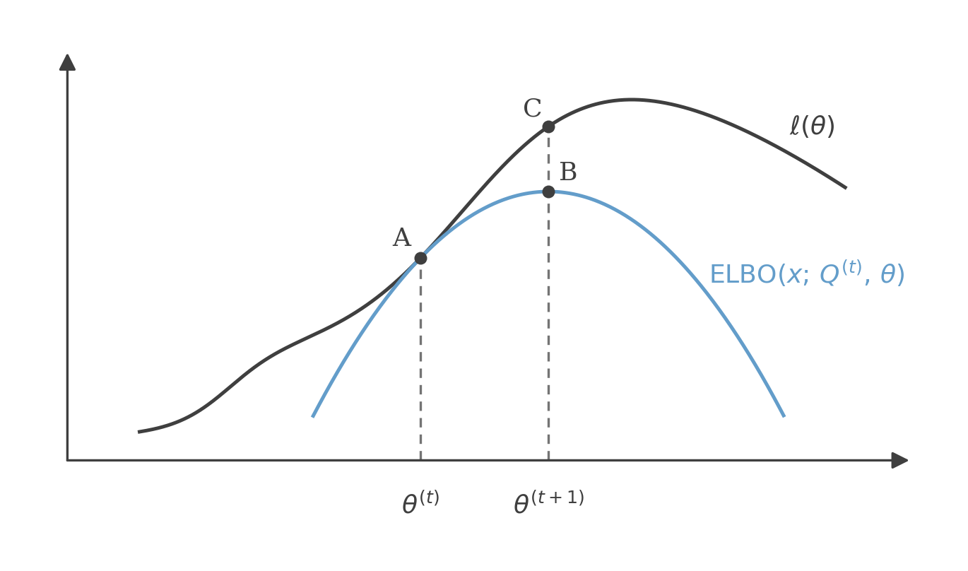
p ( z ( i ) = j ∣ x ( i ) ; θ ( t ) ) = ∑ l = 1 k p ( x ( i ) ∣ z ( i ) = l ; θ ( t ) ) p ( z ( i ) = l ; θ ( t ) ) p ( x ( i ) ∣ z ( i ) = j ; θ ( t ) ) p ( z ( i ) = j ; θ ( t ) ) The E-step choice makes the bound tight at θ ( t ) \theta^{(t)} θ ( t )
In the M-step, we hold Q ( t ) Q^{(t)} Q ( t ) θ ( t + 1 ) \theta^{(t+1)} θ ( t + 1 )
This is exact EM when the E-step computes the exact posterior and the M-step globally maximizes the fixed-Q ( t ) Q^{(t)} Q ( t )
Generalized EM may instead use any M-step that increases that objective. With an exact E-step, either version makes the observed-data log-likelihood nondecreasing, although neither guarantees a global optimum.
Monotonicity and Convergence
Each exact EM iteration guarantees that the observed-data log-likelihood does not decrease:
ℓ ( θ ( t + 1 ) ) ≥ ℓ ( θ ( t ) )
\ell(\theta^{(t+1)})
\geq
\ell(\theta^{(t)})
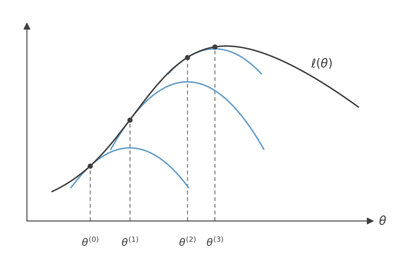
ℓ ( θ ( t + 1 ) ) ≥ ℓ ( θ ( t ) ) This does not mean that EM finds the global maximum. It may converge to a local optimum or another stationary point.
For any parameter value θ \theta θ
ℓ ( θ ) = ∑ i log p ( x ( i ) ; θ )
\ell(\theta)
=
\sum_i
\log p(x^{(i)};\theta)
ℓ ( θ ) = i ∑ log p ( x ( i ) ; θ ) is at least the sum of the per-example ELBOs.
For fixed Q t Q^{t} Q t ELBO \text{ELBO} ELBO ℓ \ell ℓ θ t \theta^{t} θ t M M M θ \theta θ θ t + 1 \theta^{t+1} θ t + 1 ℓ ≥ ELBO \ell \geq \text{ELBO} ℓ ≥ ELBO ℓ ( θ t + 1 ) \ell(\theta^{t+1}) ℓ ( θ t + 1 )
First:
ℓ ( θ ( t + 1 ) ) ≥ ∑ i = 1 n ELBO ( x ( i ) ; Q i ( t ) , θ ( t + 1 ) )
\ell(\theta^{(t+1)})
\geq
\sum_{i=1}^n
\text{ELBO}
\left(
x^{(i)};
Q_i^{(t)},
\theta^{(t+1)}
\right)
ℓ ( θ ( t + 1 ) ) ≥ i = 1 ∑ n ELBO ( x ( i ) ; Q i ( t ) , θ ( t + 1 ) ) In the M-step, θ ( t + 1 ) \theta^{(t+1)} θ ( t + 1 ) Q ( t ) Q^{(t)} Q ( t )
Therefore:
∑ i = 1 n ELBO ( x ( i ) ; Q i ( t ) , θ ( t + 1 ) )
\sum_{i=1}^n
\text{ELBO}
\left(
x^{(i)};
Q_i^{(t)},
\theta^{(t+1)}
\right)
i = 1 ∑ n ELBO ( x ( i ) ; Q i ( t ) , θ ( t + 1 ) ) ≥ ∑ i = 1 n ELBO ( x ( i ) ; Q i ( t ) , θ ( t ) )
\geq
\sum_{i=1}^n
\text{ELBO}
\left(
x^{(i)};
Q_i^{(t)},
\theta^{(t)}
\right)
≥ i = 1 ∑ n ELBO ( x ( i ) ; Q i ( t ) , θ ( t ) ) Finally, the E-step chooses Q Q Q
∑ i = 1 n ELBO ( x ( i ) ; Q i ( t ) , θ ( t ) ) = ℓ ( θ ( t ) )
\sum_{i=1}^n
\text{ELBO}
\left(
x^{(i)};
Q_i^{(t)},
\theta^{(t)}
\right)
=
\ell(\theta^{(t)})
i = 1 ∑ n ELBO ( x ( i ) ; Q i ( t ) , θ ( t ) ) = ℓ ( θ ( t ) ) Putting these together:
ℓ ( θ ( t + 1 ) ) ≥ ℓ ( θ ( t ) )
\ell(\theta^{(t+1)})
\geq
\ell(\theta^{(t)})
ℓ ( θ ( t + 1 ) ) ≥ ℓ ( θ ( t ) ) Tightness at θ ( t ) \theta^{(t)} θ ( t ) Q ( t ) Q^{(t)} Q ( t )
Additional assumptions are needed for stronger convergence claims.
In this illustrative run, each fresh bound touches ℓ \ell ℓ θ k \theta^k θ k
For an unconstrained Gaussian mixture model, the likelihood is not even bounded above: one component can collapse its covariance around a data point.
In practice, covariance constraints, regularization, or priors are used to prevent this degeneracy.
Other Interpretations
The evidence lower bound can also be written as:
ELBO ( x ; Q , θ ) = E z ∼ Q [ log p ( x , z ; θ ) ] + H ( Q )
\text{ELBO}(x;Q,\theta)
=
\mathbb{E}_{z\sim Q}
\left[
\log p(x,z;\theta)
\right]
+
H(Q)
ELBO ( x ; Q , θ ) = E z ∼ Q [ log p ( x , z ; θ ) ] + H ( Q ) where:
H ( Q ) = − E z ∼ Q [ log Q ( z ) ]
H(Q)
=
-
\mathbb{E}_{z\sim Q}
[\log Q(z)]
H ( Q ) = − E z ∼ Q [ log Q ( z )] Factoring the joint distribution gives:
ELBO ( x ; Q , θ ) = E z ∼ Q [ log p ( x ∣ z ; θ ) ] − D K L ( Q ∥ p ( z ; θ ) )
\text{ELBO}(x;Q,\theta)
=
\mathbb{E}_{z\sim Q}
\left[
\log p(x\mid z;\theta)
\right]
-
D_{KL}
\left(
Q\parallel p(z;\theta)
\right)
ELBO ( x ; Q , θ ) = E z ∼ Q [ log p ( x ∣ z ; θ ) ] − D K L ( Q ∥ p ( z ; θ ) ) If the prior p ( z ; θ ) p(z;\theta) p ( z ; θ ) θ \theta θ θ \theta θ
This is not true in general. For example, the GMM mixing weights parameterize the prior over component assignments.
› See derivationFor two distributions over a random variable z z z
D K L ( Q ∥ p ) = ∑ z Q ( z ) log Q ( z ) p ( z )
D_{KL}(Q\parallel p)
=
\sum_z
Q(z)
\log
\frac{Q(z)}{p(z)}
D K L ( Q ∥ p ) = z ∑ Q ( z ) log p ( z ) Q ( z ) = E z ∼ Q [ log Q ( z ) p ( z ) ]
=
\mathbb{E}_{z\sim Q}
\left[
\log
\frac{Q(z)}{p(z)}
\right]
= E z ∼ Q [ log p ( z ) Q ( z ) ] ELBO ( x ; Q , θ ) = E z ∼ Q [ log p ( x , z ; θ ) Q ( z ) ]
\text{ELBO}(x;Q,\theta)
=
\mathbb{E}_{z\sim Q}
\left[
\log
\frac{p(x,z;\theta)}{Q(z)}
\right]
ELBO ( x ; Q , θ ) = E z ∼ Q [ log Q ( z ) p ( x , z ; θ ) ] = E z ∼ Q [ log p ( x ∣ z ; θ ) p ( z ; θ ) Q ( z ) ]
=
\mathbb{E}_{z\sim Q}
\left[
\log
\frac{
p(x\mid z;\theta)p(z;\theta)
}{
Q(z)
}
\right]
= E z ∼ Q [ log Q ( z ) p ( x ∣ z ; θ ) p ( z ; θ ) ] = E z ∼ Q [ log p ( x ∣ z ; θ ) + log p ( z ; θ ) − log Q ( z ) ]
=
\mathbb{E}_{z\sim Q}
\left[
\log p(x\mid z;\theta)
+
\log p(z;\theta)
-
\log Q(z)
\right]
= E z ∼ Q [ log p ( x ∣ z ; θ ) + log p ( z ; θ ) − log Q ( z ) ] = E z ∼ Q [ log p ( x ∣ z ; θ ) − log Q ( z ) p ( z ; θ ) ]
=
\mathbb{E}_{z\sim Q}
\left[
\log p(x\mid z;\theta)
-
\log
\frac{Q(z)}{p(z;\theta)}
\right]
= E z ∼ Q [ log p ( x ∣ z ; θ ) − log p ( z ; θ ) Q ( z ) ] = E z ∼ Q [ log p ( x ∣ z ; θ ) ] − E z ∼ Q [ log Q ( z ) p ( z ; θ ) ]
=
\mathbb{E}_{z\sim Q}
\left[
\log p(x\mid z;\theta)
\right]
-
\mathbb{E}_{z\sim Q}
\left[
\log
\frac{Q(z)}{p(z;\theta)}
\right]
= E z ∼ Q [ log p ( x ∣ z ; θ ) ] − E z ∼ Q [ log p ( z ; θ ) Q ( z ) ] = E z ∼ Q [ log p ( x ∣ z ; θ ) ] − D K L ( Q ∥ p ( z ; θ ) )
=
\mathbb{E}_{z\sim Q}
\left[
\log p(x\mid z;\theta)
\right]
-
D_{KL}
\left(
Q\parallel p(z;\theta)
\right)
= E z ∼ Q [ log p ( x ∣ z ; θ ) ] − D K L ( Q ∥ p ( z ; θ ) ) A second useful form relates the ELBO directly to the log-likelihood:
ELBO ( x ; Q , θ ) = log p ( x ; θ ) − D K L ( Q ∥ p ( z ∣ x ; θ ) )
\text{ELBO}(x;Q,\theta)
=
\log p(x;\theta)
-
D_{KL}
\left(
Q
\parallel
p(z\mid x;\theta)
\right)
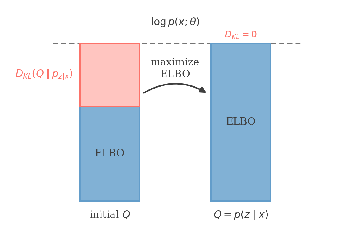
ELBO ( x ; Q , θ ) = log p ( x ; θ ) − D K L ( Q ∥ p ( z ∣ x ; θ ) ) This shows that for a fixed value of θ \theta θ
Q ( z ) = p ( z ∣ x ; θ )
Q(z)
=
p(z\mid x;\theta)
Q ( z ) = p ( z ∣ x ; θ ) because this makes the KL divergence equal to 0 0 0
This is exactly the choice made in the E-step.
At a fixed θ \theta θ log p ( x ; θ ) \log p(x;\theta) log p ( x ; θ ) ELBO \text{ELBO} ELBO D K L ( Q ∥ p ( z ∣ x ; θ ) ) D_{KL}(Q\parallel p(z\mid x;\theta)) D K L ( Q ∥ p ( z ∣ x ; θ )) Q = p ( z ∣ x ; θ ) Q=p(z\mid x;\theta) Q = p ( z ∣ x ; θ )
› See derivationELBO ( x ; Q , θ ) = E z ∼ Q [ log p ( x , z ; θ ) Q ( z ) ]
\text{ELBO}(x;Q,\theta)
=
\mathbb{E}_{z\sim Q}
\left[
\log
\frac{p(x,z;\theta)}{Q(z)}
\right]
ELBO ( x ; Q , θ ) = E z ∼ Q [ log Q ( z ) p ( x , z ; θ ) ] = E z ∼ Q [ log p ( z ∣ x ; θ ) p ( x ; θ ) Q ( z ) ]
=
\mathbb{E}_{z\sim Q}
\left[
\log
\frac{
p(z\mid x;\theta)p(x;\theta)
}{
Q(z)
}
\right]
= E z ∼ Q [ log Q ( z ) p ( z ∣ x ; θ ) p ( x ; θ ) ] = E z ∼ Q [ log p ( z ∣ x ; θ ) + log p ( x ; θ ) − log Q ( z ) ]
=
\mathbb{E}_{z\sim Q}
\left[
\log p(z\mid x;\theta)
+
\log p(x;\theta)
-
\log Q(z)
\right]
= E z ∼ Q [ log p ( z ∣ x ; θ ) + log p ( x ; θ ) − log Q ( z ) ] = E z ∼ Q [ log p ( x ; θ ) − log Q ( z ) p ( z ∣ x ; θ ) ]
=
\mathbb{E}_{z\sim Q}
\left[
\log p(x;\theta)
-
\log
\frac{Q(z)}{p(z\mid x;\theta)}
\right]
= E z ∼ Q [ log p ( x ; θ ) − log p ( z ∣ x ; θ ) Q ( z ) ] = E z ∼ Q [ log p ( x ; θ ) ] − E z ∼ Q [ log Q ( z ) p ( z ∣ x ; θ ) ]
=
\mathbb{E}_{z\sim Q}
\left[
\log p(x;\theta)
\right]
-
\mathbb{E}_{z\sim Q}
\left[
\log
\frac{Q(z)}{p(z\mid x;\theta)}
\right]
= E z ∼ Q [ log p ( x ; θ ) ] − E z ∼ Q [ log p ( z ∣ x ; θ ) Q ( z ) ] = log p ( x ; θ ) − D K L ( Q ∥ p ( z ∣ x ; θ ) )
=
\log p(x;\theta)
-
D_{KL}
\left(
Q\parallel p(z\mid x;\theta)
\right)
= log p ( x ; θ ) − D K L ( Q ∥ p ( z ∣ x ; θ ) ) Gaussian Mixture Models
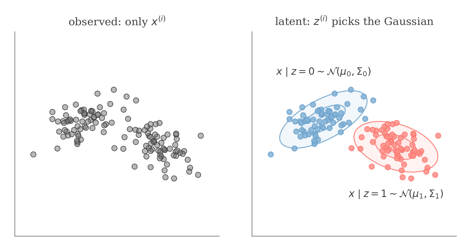
A Gaussian Mixture Model assumes that each observation comes from one of k k k
For each example x ( i ) x^{(i)} x ( i )
z ( i ) ∈ { 1 , … , k }
z^{(i)}
\in
\{1,\ldots,k\}
z ( i ) ∈ { 1 , … , k } indicating which Gaussian generated it.
First, a component is chosen according to:
p ( z ( i ) = j ) = ϕ j
p(z^{(i)}=j)
=
\phi_j
p ( z ( i ) = j ) = ϕ j where:
ϕ j > 0 , ∑ j = 1 k ϕ j = 1
\phi_j>0,
\qquad
\sum_{j=1}^k
\phi_j
=
1
ϕ j > 0 , j = 1 ∑ k ϕ j = 1 Then the observation is drawn from that component:
x ( i ) ∣ z ( i ) = j ∼ N ( μ j , Σ j )
x^{(i)}
\mid
z^{(i)}=j
\sim
\mathcal N(\mu_j,\Sigma_j)
x ( i ) ∣ z ( i ) = j ∼ N ( μ j , Σ j ) where:
μ j ∈ R d
\mu_j\in\mathbb R^d
μ j ∈ R d and:
Σ j ∈ R d × d
\Sigma_j
\in
\mathbb R^{d\times d}
Σ j ∈ R d × d is a symmetric positive-definite covariance matrix.
All we observe is the unlabeled cloud x ( i ) x^{(i)} x ( i ) z ( i ) z^{(i)} z ( i ) z ( i ) z^{(i)} z ( i )
The component labels themselves are arbitrary: permuting all component labels gives the same mixture distribution.
In practice, covariance regularization is also commonly used to prevent a component from collapsing around a single training example.
The log-likelihood is:
ℓ ( ϕ , μ , Σ ) = ∑ i = 1 n log p ( x ( i ) ; ϕ , μ , Σ )
\ell(\phi,\mu,\Sigma)
=
\sum_{i=1}^n
\log
p(x^{(i)};\phi,\mu,\Sigma)
ℓ ( ϕ , μ , Σ ) = i = 1 ∑ n log p ( x ( i ) ; ϕ , μ , Σ ) = ∑ i = 1 n log ∑ z ( i ) = 1 k p ( x ( i ) ∣ z ( i ) ; μ , Σ ) p ( z ( i ) ; ϕ )
=
\sum_{i=1}^n
\log
\sum_{z^{(i)}=1}^k
p(x^{(i)}\mid z^{(i)};\mu,\Sigma)
p(z^{(i)};\phi)
= i = 1 ∑ n log z ( i ) = 1 ∑ k p ( x ( i ) ∣ z ( i ) ; μ , Σ ) p ( z ( i ) ; ϕ ) The difficulty is that we do not know which component generated each observation.
If the z ( i ) z^{(i)} z ( i ) Gaussian Discriminant Analysis .
EM handles the missing assignments by alternating between estimating them and updating the Gaussian parameters.
Responsibilities in the E-Step
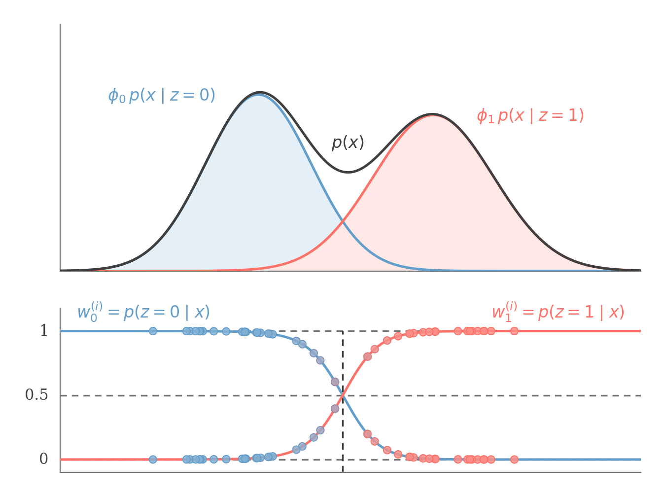
In the E-step, instead of assigning each point to exactly one component, EM gives every component a probability of having generated that point.
This probability is called a responsibility :
w j ( i ) = p ( z ( i ) = j ∣ x ( i ) ; ϕ , μ , Σ )
w_j^{(i)}
=
p
\left(
z^{(i)}=j
\mid
x^{(i)};
\phi,\mu,\Sigma
\right)
w j ( i ) = p ( z ( i ) = j ∣ x ( i ) ; ϕ , μ , Σ ) Using Bayes' rule:
w j ( i ) = p ( x ( i ) ∣ z ( i ) = j ; μ , Σ ) p ( z ( i ) = j ; ϕ ) ∑ l = 1 k p ( x ( i ) ∣ z ( i ) = l ; μ , Σ ) p ( z ( i ) = l ; ϕ )
w_j^{(i)}
=
\frac{
p(x^{(i)}\mid z^{(i)}=j;\mu,\Sigma)
p(z^{(i)}=j;\phi)
}{
\sum_{l=1}^k
p(x^{(i)}\mid z^{(i)}=l;\mu,\Sigma)
p(z^{(i)}=l;\phi)
}
w j ( i ) = ∑ l = 1 k p ( x ( i ) ∣ z ( i ) = l ; μ , Σ ) p ( z ( i ) = l ; ϕ ) p ( x ( i ) ∣ z ( i ) = j ; μ , Σ ) p ( z ( i ) = j ; ϕ ) The responsibilities for one example sum to 1 1 1
∑ j = 1 k w j ( i ) = 1
\sum_{j=1}^k
w_j^{(i)}
=
1
j = 1 ∑ k w j ( i ) = 1 After substituting the Gaussian densities, the responsibilities can also be written in a softmax-like form.
The mixture p ( x ) p(x) p ( x ) ϕ j p ( x ∣ z = j ) \phi_j p(x\mid z=j) ϕ j p ( x ∣ z = j ) w j ( i ) = p ( z = j ∣ x ( i ) ) w_j^{(i)}=p(z=j\mid x^{(i)}) w j ( i ) = p ( z = j ∣ x ( i ) ) 0 0 0 1 1 1
› See derivationp ( z ( i ) = j ∣ x ( i ) ; ϕ , μ , Σ )
p(z^{(i)}=j\mid x^{(i)};\phi,\mu,\Sigma)
p ( z ( i ) = j ∣ x ( i ) ; ϕ , μ , Σ ) = p ( x ( i ) ∣ z ( i ) = j ; μ , Σ ) p ( z ( i ) = j ; ϕ ) ∑ l = 1 k p ( x ( i ) ∣ z ( i ) = l ; μ , Σ ) p ( z ( i ) = l ; ϕ )
=
\frac{
p(x^{(i)}\mid z^{(i)}=j;\mu,\Sigma)
p(z^{(i)}=j;\phi)
}{
\sum_{l=1}^k
p(x^{(i)}\mid z^{(i)}=l;\mu,\Sigma)
p(z^{(i)}=l;\phi)
}
= ∑ l = 1 k p ( x ( i ) ∣ z ( i ) = l ; μ , Σ ) p ( z ( i ) = l ; ϕ ) p ( x ( i ) ∣ z ( i ) = j ; μ , Σ ) p ( z ( i ) = j ; ϕ ) Substituting the Gaussian densities:
= 1 ( 2 π ) d / 2 ∣ Σ j ∣ 1 / 2 exp ( − 1 2 ( x ( i ) − μ j ) T Σ j − 1 ( x ( i ) − μ j ) ) ϕ j ∑ l = 1 k [ 1 ( 2 π ) d / 2 ∣ Σ l ∣ 1 / 2 exp ( − 1 2 ( x ( i ) − μ l ) T Σ l − 1 ( x ( i ) − μ l ) ) ϕ l ]
=
\frac{
\frac{1}{(2\pi)^{d/2}|\Sigma_j|^{1/2}}
\exp
\left(
-\frac12
(x^{(i)}-\mu_j)^T
\Sigma_j^{-1}
(x^{(i)}-\mu_j)
\right)
\phi_j
}{
\sum_{l=1}^k
\left[
\frac{1}{(2\pi)^{d/2}|\Sigma_l|^{1/2}}
\exp
\left(
-\frac12
(x^{(i)}-\mu_l)^T
\Sigma_l^{-1}
(x^{(i)}-\mu_l)
\right)
\phi_l
\right]
}
= ∑ l = 1 k [ ( 2 π ) d /2 ∣ Σ l ∣ 1/2 1 exp ( − 2 1 ( x ( i ) − μ l ) T Σ l − 1 ( x ( i ) − μ l ) ) ϕ l ] ( 2 π ) d /2 ∣ Σ j ∣ 1/2 1 exp ( − 2 1 ( x ( i ) − μ j ) T Σ j − 1 ( x ( i ) − μ j ) ) ϕ j = ∣ Σ j ∣ − 1 / 2 exp ( − 1 2 ( x ( i ) − μ j ) T Σ j − 1 ( x ( i ) − μ j ) ) ϕ j ∑ l = 1 k [ ∣ Σ l ∣ − 1 / 2 exp ( − 1 2 ( x ( i ) − μ l ) T Σ l − 1 ( x ( i ) − μ l ) ) ϕ l ]
=
\frac{
|\Sigma_j|^{-1/2}
\exp
\left(
-\frac12
(x^{(i)}-\mu_j)^T
\Sigma_j^{-1}
(x^{(i)}-\mu_j)
\right)
\phi_j
}{
\sum_{l=1}^k
\left[
|\Sigma_l|^{-1/2}
\exp
\left(
-\frac12
(x^{(i)}-\mu_l)^T
\Sigma_l^{-1}
(x^{(i)}-\mu_l)
\right)
\phi_l
\right]
}
= ∑ l = 1 k [ ∣ Σ l ∣ − 1/2 exp ( − 2 1 ( x ( i ) − μ l ) T Σ l − 1 ( x ( i ) − μ l ) ) ϕ l ] ∣ Σ j ∣ − 1/2 exp ( − 2 1 ( x ( i ) − μ j ) T Σ j − 1 ( x ( i ) − μ j ) ) ϕ j i The factor ( 2 π ) − d / 2 (2\pi)^{-d/2} ( 2 π ) − d /2
Define the score:
α j ( x ( i ) ) = log ϕ j − 1 2 log ∣ Σ j ∣ − 1 2 ( x ( i ) − μ j ) T Σ j − 1 ( x ( i ) − μ j )
\alpha_j(x^{(i)})
=
\log\phi_j
-
\frac12
\log|\Sigma_j|
-
\frac12
(x^{(i)}-\mu_j)^T
\Sigma_j^{-1}
(x^{(i)}-\mu_j)
α j ( x ( i ) ) = log ϕ j − 2 1 log ∣ Σ j ∣ − 2 1 ( x ( i ) − μ j ) T Σ j − 1 ( x ( i ) − μ j ) Then:
p ( z ( i ) = j ∣ x ( i ) ; ϕ , μ , Σ ) = exp ( α j ( x ( i ) ) ) ∑ l = 1 k exp ( α l ( x ( i ) ) )
p(z^{(i)}=j\mid x^{(i)};\phi,\mu,\Sigma)
=
\frac{
\exp(\alpha_j(x^{(i)}))
}{
\sum_{l=1}^k
\exp(\alpha_l(x^{(i)}))
}
p ( z ( i ) = j ∣ x ( i ) ; ϕ , μ , Σ ) = ∑ l = 1 k exp ( α l ( x ( i ) )) exp ( α j ( x ( i ) )) To verify this:
exp ( α j ( x ( i ) ) ) ∑ l = 1 k exp ( α l ( x ( i ) ) )
\frac{
\exp(\alpha_j(x^{(i)}))
}{
\sum_{l=1}^k
\exp(\alpha_l(x^{(i)}))
}
∑ l = 1 k exp ( α l ( x ( i ) )) exp ( α j ( x ( i ) )) = exp ( log ϕ j − 1 2 log ∣ Σ j ∣ − 1 2 ( x ( i ) − μ j ) T Σ j − 1 ( x ( i ) − μ j ) ) ∑ l = 1 k exp ( log ϕ l − 1 2 log ∣ Σ l ∣ − 1 2 ( x ( i ) − μ l ) T Σ l − 1 ( x ( i ) − μ l ) )
=
\frac{
\exp
\left(
\log\phi_j
-
\frac12\log|\Sigma_j|
-
\frac12
(x^{(i)}-\mu_j)^T
\Sigma_j^{-1}
(x^{(i)}-\mu_j)
\right)
}{
\sum_{l=1}^k
\exp
\left(
\log\phi_l
-
\frac12\log|\Sigma_l|
-
\frac12
(x^{(i)}-\mu_l)^T
\Sigma_l^{-1}
(x^{(i)}-\mu_l)
\right)
}
= ∑ l = 1 k exp ( log ϕ l − 2 1 log ∣ Σ l ∣ − 2 1 ( x ( i ) − μ l ) T Σ l − 1 ( x ( i ) − μ l ) ) exp ( log ϕ j − 2 1 log ∣ Σ j ∣ − 2 1 ( x ( i ) − μ j ) T Σ j − 1 ( x ( i ) − μ j ) ) = ϕ j exp ( − 1 2 log ∣ Σ j ∣ − 1 2 ( x ( i ) − μ j ) T Σ j − 1 ( x ( i ) − μ j ) ) ∑ l = 1 k ϕ l exp ( − 1 2 log ∣ Σ l ∣ − 1 2 ( x ( i ) − μ l ) T Σ l − 1 ( x ( i ) − μ l ) )
=
\frac{
\phi_j
\exp
\left(
-\frac12\log|\Sigma_j|
-
\frac12
(x^{(i)}-\mu_j)^T
\Sigma_j^{-1}
(x^{(i)}-\mu_j)
\right)
}{
\sum_{l=1}^k
\phi_l
\exp
\left(
-\frac12\log|\Sigma_l|
-
\frac12
(x^{(i)}-\mu_l)^T
\Sigma_l^{-1}
(x^{(i)}-\mu_l)
\right)
}
= ∑ l = 1 k ϕ l exp ( − 2 1 log ∣ Σ l ∣ − 2 1 ( x ( i ) − μ l ) T Σ l − 1 ( x ( i ) − μ l ) ) ϕ j exp ( − 2 1 log ∣ Σ j ∣ − 2 1 ( x ( i ) − μ j ) T Σ j − 1 ( x ( i ) − μ j ) ) = ∣ Σ j ∣ − 1 / 2 exp ( − 1 2 ( x ( i ) − μ j ) T Σ j − 1 ( x ( i ) − μ j ) ) ϕ j ∑ l = 1 k [ ∣ Σ l ∣ − 1 / 2 exp ( − 1 2 ( x ( i ) − μ l ) T Σ l − 1 ( x ( i ) − μ l ) ) ϕ l ]
=
\frac{
|\Sigma_j|^{-1/2}
\exp
\left(
-\frac12
(x^{(i)}-\mu_j)^T
\Sigma_j^{-1}
(x^{(i)}-\mu_j)
\right)
\phi_j
}{
\sum_{l=1}^k
\left[
|\Sigma_l|^{-1/2}
\exp
\left(
-\frac12
(x^{(i)}-\mu_l)^T
\Sigma_l^{-1}
(x^{(i)}-\mu_l)
\right)
\phi_l
\right]
}
= ∑ l = 1 k [ ∣ Σ l ∣ − 1/2 exp ( − 2 1 ( x ( i ) − μ l ) T Σ l − 1 ( x ( i ) − μ l ) ) ϕ l ] ∣ Σ j ∣ − 1/2 exp ( − 2 1 ( x ( i ) − μ j ) T Σ j − 1 ( x ( i ) − μ j ) ) ϕ j i Using exp ( b log a ) = a b \exp(b\log a)=a^b exp ( b log a ) = a b
Parameter Updates in the M-Step
In the M-step, the responsibilities w j ( i ) w_j^{(i)} w j ( i )
The resulting updates are responsibility-weighted versions of the usual sample estimates:
ϕ l = 1 n ∑ i = 1 n w l ( i )
\phi_l
=
\frac1n
\sum_{i=1}^n
w_l^{(i)}
ϕ l = n 1 i = 1 ∑ n w l ( i ) μ l = ∑ i = 1 n w l ( i ) x ( i ) ∑ i = 1 n w l ( i )
\mu_l
=
\frac{
\sum_{i=1}^n
w_l^{(i)}x^{(i)}
}{
\sum_{i=1}^n
w_l^{(i)}
}
μ l = ∑ i = 1 n w l ( i ) ∑ i = 1 n w l ( i ) x ( i ) Σ l = ∑ i = 1 n w l ( i ) ( x ( i ) − μ l ) ( x ( i ) − μ l ) T ∑ i = 1 n w l ( i )
\Sigma_l
=
\frac{
\sum_{i=1}^n
w_l^{(i)}
(x^{(i)}-\mu_l)
(x^{(i)}-\mu_l)^T
}{
\sum_{i=1}^n
w_l^{(i)}
}
Σ l = ∑ i = 1 n w l ( i ) ∑ i = 1 n w l ( i ) ( x ( i ) − μ l ) ( x ( i ) − μ l ) T So each component is fitted as if every observation belonged to it partially, with weight w l ( i ) w_l^{(i)} w l ( i )
These updates come from maximizing the fixed-responsibility ELBO:
∑ i = 1 n ∑ j = 1 k w j ( i ) log p ( x ( i ) ∣ z ( i ) = j ; μ , Σ ) p ( z ( i ) = j ; ϕ ) w j ( i )
\sum_{i=1}^{n}
\sum_{j=1}^{k}
w_j^{(i)}
\log
\frac{
p(x^{(i)}\mid z^{(i)}=j;\mu,\Sigma)
p(z^{(i)}=j;\phi)
}{
w_j^{(i)}
}
i = 1 ∑ n j = 1 ∑ k w j ( i ) log w j ( i ) p ( x ( i ) ∣ z ( i ) = j ; μ , Σ ) p ( z ( i ) = j ; ϕ ) › See derivationStart with:
∑ i = 1 n ∑ j = 1 k w j ( i ) log p ( x ( i ) ∣ z ( i ) = j ; μ , Σ ) p ( z ( i ) = j ; ϕ ) w j ( i )
\sum_{i=1}^{n}
\sum_{j=1}^{k}
w_j^{(i)}
\log
\frac{
p(x^{(i)}\mid z^{(i)}=j;\mu,\Sigma)
p(z^{(i)}=j;\phi)
}{
w_j^{(i)}
}
i = 1 ∑ n j = 1 ∑ k w j ( i ) log w j ( i ) p ( x ( i ) ∣ z ( i ) = j ; μ , Σ ) p ( z ( i ) = j ; ϕ ) Substituting the Gaussian density:
= ∑ i = 1 n ∑ j = 1 k w j ( i ) log ( 1 ( 2 π ) d / 2 ∣ Σ j ∣ 1 / 2 exp ( − 1 2 ( x ( i ) − μ j ) T Σ j − 1 ( x ( i ) − μ j ) ) ϕ j w j ( i ) )
=
\sum_{i=1}^n
\sum_{j=1}^k
w_j^{(i)}
\log
\left(
\frac{
\frac{1}{(2\pi)^{d/2}|\Sigma_j|^{1/2}}
\exp
\left(
-\frac12
(x^{(i)}-\mu_j)^T
\Sigma_j^{-1}
(x^{(i)}-\mu_j)
\right)
\phi_j
}{
w_j^{(i)}
}
\right)
= i = 1 ∑ n j = 1 ∑ k w j ( i ) log ( w j ( i ) ( 2 π ) d /2 ∣ Σ j ∣ 1/2 1 exp ( − 2 1 ( x ( i ) − μ j ) T Σ j − 1 ( x ( i ) − μ j ) ) ϕ j ) = ∑ i = 1 n ∑ j = 1 k w j ( i ) [ log ( 1 ( 2 π ) d / 2 ∣ Σ j ∣ 1 / 2 ) − 1 2 ( x ( i ) − μ j ) T Σ j − 1 ( x ( i ) − μ j ) + log ϕ j − log w j ( i ) ]
=
\sum_{i=1}^n
\sum_{j=1}^k
w_j^{(i)}
\left[
\log
\left(
\frac{1}{(2\pi)^{d/2}|\Sigma_j|^{1/2}}
\right)
-
\frac12
(x^{(i)}-\mu_j)^T
\Sigma_j^{-1}
(x^{(i)}-\mu_j)
+
\log\phi_j
-
\log w_j^{(i)}
\right]
= i = 1 ∑ n j = 1 ∑ k w j ( i ) [ log ( ( 2 π ) d /2 ∣ Σ j ∣ 1/2 1 ) − 2 1 ( x ( i ) − μ j ) T Σ j − 1 ( x ( i ) − μ j ) + log ϕ j − log w j ( i ) ] First, take the derivative with respect to μ l \mu_l μ l
∇ μ l ∑ i = 1 n ∑ j = 1 k w j ( i ) [ − 1 2 ( x ( i ) − μ j ) T Σ j − 1 ( x ( i ) − μ j ) ]
\nabla_{\mu_l}
\sum_{i=1}^n
\sum_{j=1}^k
w_j^{(i)}
\left[
-\frac12
(x^{(i)}-\mu_j)^T
\Sigma_j^{-1}
(x^{(i)}-\mu_j)
\right]
∇ μ l i = 1 ∑ n j = 1 ∑ k w j ( i ) [ − 2 1 ( x ( i ) − μ j ) T Σ j − 1 ( x ( i ) − μ j ) ] = ∑ i = 1 n w l ( i ) ∇ μ l [ − 1 2 ( x ( i ) − μ l ) T Σ l − 1 ( x ( i ) − μ l ) ]
=
\sum_{i=1}^n
w_l^{(i)}
\nabla_{\mu_l}
\left[
-\frac12
(x^{(i)}-\mu_l)^T
\Sigma_l^{-1}
(x^{(i)}-\mu_l)
\right]
= i = 1 ∑ n w l ( i ) ∇ μ l [ − 2 1 ( x ( i ) − μ l ) T Σ l − 1 ( x ( i ) − μ l ) ] i All terms with j ≠ l j\neq l j = l μ l \mu_l μ l
Expanding the quadratic term:
= ∑ i = 1 n w l ( i ) ∇ μ l [ − 1 2 ( x ( i ) T Σ l − 1 x ( i ) − μ l T Σ l − 1 x ( i ) − x ( i ) T Σ l − 1 μ l + μ l T Σ l − 1 μ l ) ]
=
\sum_{i=1}^n
w_l^{(i)}
\nabla_{\mu_l}
\left[
-\frac12
\left(
x^{(i)T}\Sigma_l^{-1}x^{(i)}
-
\mu_l^T\Sigma_l^{-1}x^{(i)}
-
x^{(i)T}\Sigma_l^{-1}\mu_l
+
\mu_l^T\Sigma_l^{-1}\mu_l
\right)
\right]
= i = 1 ∑ n w l ( i ) ∇ μ l [ − 2 1 ( x ( i ) T Σ l − 1 x ( i ) − μ l T Σ l − 1 x ( i ) − x ( i ) T Σ l − 1 μ l + μ l T Σ l − 1 μ l ) ] = ∑ i = 1 n w l ( i ) [ − 1 2 ( − Σ l − 1 x ( i ) − Σ l − T x ( i ) + 2 Σ l − 1 μ l ) ]
=
\sum_{i=1}^n
w_l^{(i)}
\left[
-\frac12
\left(
-\Sigma_l^{-1}x^{(i)}
-
\Sigma_l^{-T}x^{(i)}
+
2\Sigma_l^{-1}\mu_l
\right)
\right]
= i = 1 ∑ n w l ( i ) [ − 2 1 ( − Σ l − 1 x ( i ) − Σ l − T x ( i ) + 2 Σ l − 1 μ l ) ] i For a symmetric matrix A A A ∇ x ( x T A x ) = 2 A x \nabla_x(x^TAx)=2Ax ∇ x ( x T A x ) = 2 A x
= ∑ i = 1 n w l ( i ) [ − 1 2 ( − Σ l − 1 x ( i ) − Σ l − 1 x ( i ) + 2 Σ l − 1 μ l ) ]
=
\sum_{i=1}^n
w_l^{(i)}
\left[
-\frac12
\left(
-\Sigma_l^{-1}x^{(i)}
-
\Sigma_l^{-1}x^{(i)}
+
2\Sigma_l^{-1}\mu_l
\right)
\right]
= i = 1 ∑ n w l ( i ) [ − 2 1 ( − Σ l − 1 x ( i ) − Σ l − 1 x ( i ) + 2 Σ l − 1 μ l ) ] i Since Σ l \Sigma_l Σ l Σ l − T = Σ l − 1 \Sigma_l^{-T}=\Sigma_l^{-1} Σ l − T = Σ l − 1
Therefore:
= ∑ i = 1 n w l ( i ) ( Σ l − 1 x ( i ) − Σ l − 1 μ l )
=
\sum_{i=1}^n
w_l^{(i)}
\left(
\Sigma_l^{-1}x^{(i)}
-
\Sigma_l^{-1}\mu_l
\right)
= i = 1 ∑ n w l ( i ) ( Σ l − 1 x ( i ) − Σ l − 1 μ l ) Setting this equal to 0 0 0
∑ i = 1 n w l ( i ) Σ l − 1 x ( i ) = ∑ i = 1 n w l ( i ) Σ l − 1 μ l
\sum_{i=1}^n
w_l^{(i)}
\Sigma_l^{-1}x^{(i)}
=
\sum_{i=1}^n
w_l^{(i)}
\Sigma_l^{-1}\mu_l
i = 1 ∑ n w l ( i ) Σ l − 1 x ( i ) = i = 1 ∑ n w l ( i ) Σ l − 1 μ l Σ l − 1 [ ∑ i = 1 n w l ( i ) x ( i ) ] = Σ l − 1 [ ∑ i = 1 n w l ( i ) ] μ l
\Sigma_l^{-1}
\left[
\sum_{i=1}^n
w_l^{(i)}x^{(i)}
\right]
=
\Sigma_l^{-1}
\left[
\sum_{i=1}^n
w_l^{(i)}
\right]
\mu_l
Σ l − 1 [ i = 1 ∑ n w l ( i ) x ( i ) ] = Σ l − 1 [ i = 1 ∑ n w l ( i ) ] μ l i Σ l − 1 \Sigma_l^{-1} Σ l − 1 μ l \mu_l μ l i i i
Canceling Σ l − 1 \Sigma_l^{-1} Σ l − 1
∑ i = 1 n w l ( i ) x ( i ) = [ ∑ i = 1 n w l ( i ) ] μ l
\sum_{i=1}^n
w_l^{(i)}x^{(i)}
=
\left[
\sum_{i=1}^n
w_l^{(i)}
\right]
\mu_l
i = 1 ∑ n w l ( i ) x ( i ) = [ i = 1 ∑ n w l ( i ) ] μ l Therefore:
μ l = ∑ i = 1 n w l ( i ) x ( i ) ∑ i = 1 n w l ( i )
\mu_l
=
\frac{
\sum_{i=1}^n
w_l^{(i)}x^{(i)}
}{
\sum_{i=1}^n
w_l^{(i)}
}
μ l = ∑ i = 1 n w l ( i ) ∑ i = 1 n w l ( i ) x ( i ) Now take the derivative with respect to ϕ l \phi_l ϕ l
Only the terms:
∑ i = 1 n ∑ j = 1 k w j ( i ) log ϕ j
\sum_{i=1}^n
\sum_{j=1}^k
w_j^{(i)}
\log\phi_j
i = 1 ∑ n j = 1 ∑ k w j ( i ) log ϕ j depend on ϕ \phi ϕ
Because:
∑ j = 1 k ϕ j = 1
\sum_{j=1}^k
\phi_j
=
1
j = 1 ∑ k ϕ j = 1 we use a Lagrange multiplier:
L ( ϕ ) = ∑ i = 1 n ∑ j = 1 k w j ( i ) log ϕ j + β ( ∑ j = 1 k ϕ j − 1 )
\mathcal L(\phi)
=
\sum_{i=1}^n
\sum_{j=1}^k
w_j^{(i)}
\log\phi_j
+
\beta
\left(
\sum_{j=1}^k
\phi_j
-
1
\right)
L ( ϕ ) = i = 1 ∑ n j = 1 ∑ k w j ( i ) log ϕ j + β ( j = 1 ∑ k ϕ j − 1 ) Taking the derivative:
∂ ∂ ϕ l L ( ϕ ) = ∑ i = 1 n w l ( i ) ϕ l + β
\frac{\partial}{\partial\phi_l}
\mathcal L(\phi)
=
\sum_{i=1}^n
\frac{w_l^{(i)}}{\phi_l}
+
\beta
∂ ϕ l ∂ L ( ϕ ) = i = 1 ∑ n ϕ l w l ( i ) + β Setting this equal to 0 0 0
∑ i = 1 n w l ( i ) ϕ l + β = 0
\sum_{i=1}^n
\frac{w_l^{(i)}}{\phi_l}
+
\beta
=
0
i = 1 ∑ n ϕ l w l ( i ) + β = 0 ϕ l = ∑ i = 1 n w l ( i ) − β
\phi_l
=
\frac{
\sum_{i=1}^n
w_l^{(i)}
}{
-\beta
}
ϕ l = − β ∑ i = 1 n w l ( i ) Using the constraint:
∑ j = 1 k ϕ j = 1
\sum_{j=1}^k
\phi_j
=
1
j = 1 ∑ k ϕ j = 1 gives:
∑ j = 1 k ∑ i = 1 n w j ( i ) − β = 1
\sum_{j=1}^k
\frac{
\sum_{i=1}^n
w_j^{(i)}
}{
-\beta
}
=
1
j = 1 ∑ k − β ∑ i = 1 n w j ( i ) = 1 ∑ i = 1 n ∑ j = 1 k w j ( i ) = − β
\sum_{i=1}^n
\sum_{j=1}^k
w_j^{(i)}
=
-\beta
i = 1 ∑ n j = 1 ∑ k w j ( i ) = − β ∑ i = 1 n 1 = − β
\sum_{i=1}^n
1
=
-\beta
i = 1 ∑ n 1 = − β i For each training example, the responsibilities sum to 1 1 1
Therefore:
− β = n
-\beta=n
− β = n and:
ϕ l = 1 n ∑ i = 1 n w l ( i )
\phi_l
=
\frac1n
\sum_{i=1}^n
w_l^{(i)}
ϕ l = n 1 i = 1 ∑ n w l ( i ) We use the following matrix derivatives:
∇ A ∣ A ∣ = ∣ A ∣ ( A − 1 ) T
\nabla_A|A|
=
|A|(A^{-1})^T
∇ A ∣ A ∣ = ∣ A ∣ ( A − 1 ) T and:
∇ A ( x T A − 1 x ) = − A − T x x T A − T
\nabla_A
\left(
x^TA^{-1}x
\right)
=
-A^{-T}xx^TA^{-T}
∇ A ( x T A − 1 x ) = − A − T x x T A − T When A A A
A − T = A − 1
A^{-T}=A^{-1}
A − T = A − 1 Finally, take the derivative with respect to Σ l \Sigma_l Σ l
∇ Σ l ∑ i = 1 n ∑ j = 1 k w j ( i ) [ log 1 ( 2 π ) d / 2 ∣ Σ j ∣ 1 / 2 − 1 2 ( x ( i ) − μ j ) T Σ j − 1 ( x ( i ) − μ j ) ]
\nabla_{\Sigma_l}
\sum_{i=1}^n
\sum_{j=1}^k
w_j^{(i)}
\left[
\log
\frac{1}{(2\pi)^{d/2}|\Sigma_j|^{1/2}}
-
\frac12
(x^{(i)}-\mu_j)^T
\Sigma_j^{-1}
(x^{(i)}-\mu_j)
\right]
∇ Σ l i = 1 ∑ n j = 1 ∑ k w j ( i ) [ log ( 2 π ) d /2 ∣ Σ j ∣ 1/2 1 − 2 1 ( x ( i ) − μ j ) T Σ j − 1 ( x ( i ) − μ j ) ] = ∑ i = 1 n w l ( i ) ∇ Σ l [ − log ∣ Σ l ∣ 1 / 2 − 1 2 ( x ( i ) − μ l ) T Σ l − 1 ( x ( i ) − μ l ) ]
=
\sum_{i=1}^n
w_l^{(i)}
\nabla_{\Sigma_l}
\left[
-\log|\Sigma_l|^{1/2}
-
\frac12
(x^{(i)}-\mu_l)^T
\Sigma_l^{-1}
(x^{(i)}-\mu_l)
\right]
= i = 1 ∑ n w l ( i ) ∇ Σ l [ − log ∣ Σ l ∣ 1/2 − 2 1 ( x ( i ) − μ l ) T Σ l − 1 ( x ( i ) − μ l ) ] i All terms with j ≠ l j\neq l j = l Σ l \Sigma_l Σ l
We evaluate the two derivatives separately.
First:
∇ Σ l log ∣ Σ l ∣ 1 / 2
\nabla_{\Sigma_l}
\log|\Sigma_l|^{1/2}
∇ Σ l log ∣ Σ l ∣ 1/2 = 1 ∣ Σ l ∣ 1 / 2 ∇ Σ l ∣ Σ l ∣ 1 / 2
=
\frac{1}{|\Sigma_l|^{1/2}}
\nabla_{\Sigma_l}
|\Sigma_l|^{1/2}
= ∣ Σ l ∣ 1/2 1 ∇ Σ l ∣ Σ l ∣ 1/2 = 1 ∣ Σ l ∣ 1 / 2 ( 1 2 ∣ Σ l ∣ − 1 / 2 ) ∇ Σ l ∣ Σ l ∣
=
\frac{1}{|\Sigma_l|^{1/2}}
\left(
\frac12
|\Sigma_l|^{-1/2}
\right)
\nabla_{\Sigma_l}
|\Sigma_l|
= ∣ Σ l ∣ 1/2 1 ( 2 1 ∣ Σ l ∣ − 1/2 ) ∇ Σ l ∣ Σ l ∣ = 1 2 ( 1 ∣ Σ l ∣ ∣ Σ l ∣ ) Σ l − 1
=
\frac12
\left(
\frac{1}{|\Sigma_l|}
|\Sigma_l|
\right)
\Sigma_l^{-1}
= 2 1 ( ∣ Σ l ∣ 1 ∣ Σ l ∣ ) Σ l − 1 i Using ∇ A ∣ A ∣ = ∣ A ∣ ( A − 1 ) T \nabla_A|A|=|A|(A^{-1})^T ∇ A ∣ A ∣ = ∣ A ∣ ( A − 1 ) T Σ l \Sigma_l Σ l
= 1 2 Σ l − 1
=
\frac12
\Sigma_l^{-1}
= 2 1 Σ l − 1 For the quadratic term:
∇ Σ l [ ( x ( i ) − μ l ) T Σ l − 1 ( x ( i ) − μ l ) ]
\nabla_{\Sigma_l}
\left[
(x^{(i)}-\mu_l)^T
\Sigma_l^{-1}
(x^{(i)}-\mu_l)
\right]
∇ Σ l [ ( x ( i ) − μ l ) T Σ l − 1 ( x ( i ) − μ l ) ] = − Σ l − 1 ( x ( i ) − μ l ) ( x ( i ) − μ l ) T Σ l − 1
=
-
\Sigma_l^{-1}
(x^{(i)}-\mu_l)
(x^{(i)}-\mu_l)^T
\Sigma_l^{-1}
= − Σ l − 1 ( x ( i ) − μ l ) ( x ( i ) − μ l ) T Σ l − 1 Putting these together:
∑ i = 1 n w l ( i ) [ 1 2 ( − Σ l − 1 + Σ l − 1 ( x ( i ) − μ l ) ( x ( i ) − μ l ) T Σ l − 1 ) ]
\sum_{i=1}^n
w_l^{(i)}
\left[
\frac12
\left(
-\Sigma_l^{-1}
+
\Sigma_l^{-1}
(x^{(i)}-\mu_l)
(x^{(i)}-\mu_l)^T
\Sigma_l^{-1}
\right)
\right]
i = 1 ∑ n w l ( i ) [ 2 1 ( − Σ l − 1 + Σ l − 1 ( x ( i ) − μ l ) ( x ( i ) − μ l ) T Σ l − 1 ) ] Setting this equal to 0 0 0
∑ i = 1 n w l ( i ) Σ l − 1 = ∑ i = 1 n w l ( i ) Σ l − 1 ( x ( i ) − μ l ) ( x ( i ) − μ l ) T Σ l − 1
\sum_{i=1}^n
w_l^{(i)}
\Sigma_l^{-1}
=
\sum_{i=1}^n
w_l^{(i)}
\Sigma_l^{-1}
(x^{(i)}-\mu_l)
(x^{(i)}-\mu_l)^T
\Sigma_l^{-1}
i = 1 ∑ n w l ( i ) Σ l − 1 = i = 1 ∑ n w l ( i ) Σ l − 1 ( x ( i ) − μ l ) ( x ( i ) − μ l ) T Σ l − 1 ( ∑ i = 1 n w l ( i ) ) Σ l − 1 = Σ l − 1 [ ∑ i = 1 n w l ( i ) ( x ( i ) − μ l ) ( x ( i ) − μ l ) T ] Σ l − 1
\left(
\sum_{i=1}^n
w_l^{(i)}
\right)
\Sigma_l^{-1}
=
\Sigma_l^{-1}
\left[
\sum_{i=1}^n
w_l^{(i)}
(x^{(i)}-\mu_l)
(x^{(i)}-\mu_l)^T
\right]
\Sigma_l^{-1}
( i = 1 ∑ n w l ( i ) ) Σ l − 1 = Σ l − 1 [ i = 1 ∑ n w l ( i ) ( x ( i ) − μ l ) ( x ( i ) − μ l ) T ] Σ l − 1 i Σ l − 1 \Sigma_l^{-1} Σ l − 1 i i i w l ( i ) w_l^{(i)} w l ( i )
Multiplying through by Σ l \Sigma_l Σ l
Σ l ( ∑ i = 1 n w l ( i ) ) = ∑ i = 1 n w l ( i ) ( x ( i ) − μ l ) ( x ( i ) − μ l ) T
\Sigma_l
\left(
\sum_{i=1}^n
w_l^{(i)}
\right)
=
\sum_{i=1}^n
w_l^{(i)}
(x^{(i)}-\mu_l)
(x^{(i)}-\mu_l)^T
Σ l ( i = 1 ∑ n w l ( i ) ) = i = 1 ∑ n w l ( i ) ( x ( i ) − μ l ) ( x ( i ) − μ l ) T Therefore:
Σ l = ∑ i = 1 n w l ( i ) ( x ( i ) − μ l ) ( x ( i ) − μ l ) T ∑ i = 1 n w l ( i )
\Sigma_l
=
\frac{
\sum_{i=1}^n
w_l^{(i)}
(x^{(i)}-\mu_l)
(x^{(i)}-\mu_l)^T
}{
\sum_{i=1}^n
w_l^{(i)}
}
Σ l = ∑ i = 1 n w l ( i ) ∑ i = 1 n w l ( i ) ( x ( i ) − μ l ) ( x ( i ) − μ l ) T Repeat until convergence {
\text{Repeat until convergence \{}
Repeat until convergence { (E-step) For each i and j , set {
\quad
\text{(E-step) For each }i\text{ and }j,\text{ set \{}
(E-step) For each i and j , set { w j ( i ) ← p ( z ( i ) = j ∣ x ( i ) ; ϕ , μ , Σ )
\quad\quad
w_j^{(i)}
\leftarrow
p
\left(
z^{(i)}=j
\mid
x^{(i)};
\phi,\mu,\Sigma
\right)
w j ( i ) ← p ( z ( i ) = j ∣ x ( i ) ; ϕ , μ , Σ ) }
\quad
\text{\}}
} (M-step) For each j , set {
\quad
\text{(M-step) For each }j,\text{ set \{}
(M-step) For each j , set { ϕ j ← 1 n ∑ i = 1 n w j ( i )
\quad\quad
\phi_j
\leftarrow
\frac1n
\sum_{i=1}^n
w_j^{(i)}
ϕ j ← n 1 i = 1 ∑ n w j ( i ) μ j ← ∑ i = 1 n w j ( i ) x ( i ) ∑ i = 1 n w j ( i )
\quad\quad
\mu_j
\leftarrow
\frac{
\sum_{i=1}^n
w_j^{(i)}x^{(i)}
}{
\sum_{i=1}^n
w_j^{(i)}
}
μ j ← ∑ i = 1 n w j ( i ) ∑ i = 1 n w j ( i ) x ( i ) Σ j ← ∑ i = 1 n w j ( i ) ( x ( i ) − μ j ) ( x ( i ) − μ j ) T ∑ i = 1 n w j ( i )
\quad\quad
\Sigma_j
\leftarrow
\frac{
\sum_{i=1}^n
w_j^{(i)}
(x^{(i)}-\mu_j)
(x^{(i)}-\mu_j)^T
}{
\sum_{i=1}^n
w_j^{(i)}
}
Σ j ← ∑ i = 1 n w j ( i ) ∑ i = 1 n w j ( i ) ( x ( i ) − μ j ) ( x ( i ) − μ j ) T }
\quad
\text{\}}
} }
\text{\}}
} It is useful to define the effective number of examples assigned to component j j j
N j = ∑ i = 1 n w j ( i )
N_j
=
\sum_{i=1}^n
w_j^{(i)}
N j = i = 1 ∑ n w j ( i ) Because the assignments are soft, N j N_j N j
The M-step then sets:
ϕ j = N j n
\phi_j
=
\frac{N_j}{n}
ϕ j = n N j and computes responsibility-weighted means and covariances.
The responsibilities stay fixed throughout the M-step.
The E-step makes the ELBO equal to log p ( x ; θ ( t ) ) \log p(x;\theta^{(t)}) log p ( x ; θ ( t ) ) θ ( t + 1 ) \theta^{(t+1)} θ ( t + 1 )