Decision Trees and Ensembles

Introduction

A decision tree makes predictions by repeatedly splitting the data into smaller groups.

At each split, it tries to separate the training examples so that the resulting groups contain examples with similar labels.

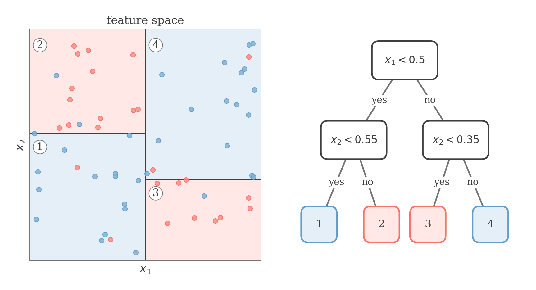
Decision tree beside the axis-aligned partition of the feature space its splits produce — Each split divides the feature space into smaller regions. Each leaf of the tree corresponds to one of these regions and produces a final prediction.

Impurity and Split Selection

To decide which split is best, we need a way to measure how mixed the labels are at a node. This is called impurity.

A pure node contains examples from only one class. A highly impure node contains a mixture of classes.

Two common impurity measures are Gini impurity and entropy.

Suppose a node contains a set of training examples $S$ . Let $p_k$ be the fraction of examples in the node that belong to class $k$ :

p_k = \frac{|S_k|}{|S|}

Gini impurity is small when most examples belong to one class and large when the classes are mixed:

G(S) = \sum_{k=1}^c p_k(1-p_k)

If the node is completely pure, one class has proportion $1$ and all others have proportion $0$ , so:

G(S)=0

Entropy measures the same general idea: how uncertain the class label is within the node.

H(S) = - \sum_{k=1}^c p_k\log p_k

We define $0\log0=0$ .

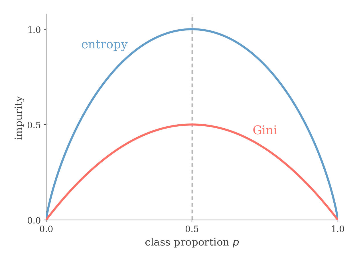
Both Gini impurity and entropy are $0$ for a pure node and largest when the classes are evenly represented.

Binary Gini and entropy impurity as a function of one class proportion, both peaking at one half — In binary classification, both Gini impurity and entropy are $0$ at a pure node and largest when the two classes are equally represented.

A candidate split divides the examples at a node into a left child $S_L$ and a right child $S_R$ .

For either impurity measure $I$ , the weighted impurity after the split is:

I_{\mathrm{split}} = \frac{|S_L|}{|S|} I(S_L) + \frac{|S_R|}{|S|} I(S_R)

The gain from the split is the reduction in impurity:

\Delta I = I(S) - I_{\mathrm{split}}

A greedy decision tree chooses the split with the largest gain, or equivalently the smallest weighted child impurity.

Entropy also has an information-theoretic interpretation. Relative to the uniform class distribution, lower entropy corresponds to larger KL divergence.

See derivation

Let $q$ be the uniform distribution over the $c$ classes:

q_i = \frac{1}{c}

Then:

D_{KL}(p\|q) = \sum_{i=1}^c p_i \log \frac{p_i}{q_i}

= \sum_{i=1}^c \left( p_i\log p_i - p_i\log\frac{1}{c} \right)

= \sum_{i=1}^c p_i\log p_i + \log c \sum_{i=1}^c p_i

= \sum_{i=1}^c p_i\log p_i + \log c

Therefore:

\arg\max_p D_{KL}(p\|q) = \arg\max_p \left[ \sum_{i=1}^c p_i\log p_i + \log c \right]

= \arg\max_p \sum_{i=1}^c p_i\log p_i

= \arg\min_p \left( - \sum_{i=1}^c p_i\log p_i \right)

= \arg\min_p H(p)

Building a Tree

Decision trees are usually built greedily: at each node, we choose the best split available at that moment and then repeat the process on each child.

This does not guarantee the globally best tree, but it makes training practical.

For a numerical feature $x_j$ , a split chooses a threshold $t$ .

Examples with:

x_j\leq t

go to the left child, while examples with:

x_j>t

go to the right child.

Therefore:

S_L(j,t) = \{(x,y)\in S:x_j\leq t\}

S_R(j,t) = \{(x,y)\in S:x_j>t\}

Suppose the distinct observed values of feature $j$ are:

v_1<v_2<\cdots<v_r

We only need to consider thresholds between consecutive values:

\mathcal{T}_j = \left\{ \frac{v_l+v_{l+1}}{2} : l=1,\ldots,r-1 \right\}

For a candidate feature $j$ and threshold $t$ , the gain is:

\Delta I(j,t) = I(S) - \frac{|S_L(j,t)|}{|S|} I(S_L(j,t)) - \frac{|S_R(j,t)|}{|S|} I(S_R(j,t))

The greedy split is:

(j^*,t^*) \in \arg\max_{j,\;t\in\mathcal T_j} \Delta I(j,t)

If we keep splitting until every leaf is pure, the tree can become very large and overfit the training data.

Common stopping rules include a maximum depth, a minimum number of examples per node or leaf, and a minimum required gain.

We can also prune a tree after training by removing branches that do not improve generalization.

At a classification leaf, we estimate the class probabilities using the class proportions within that leaf:

\widehat p(y=k\mid \text{leaf }S) = \frac{|S_k|}{|S|}

The predicted class is usually the majority class:

\widehat y = \arg\max_k |S_k|

Decision trees can also be used for regression.

The splitting process is the same, but instead of measuring class impurity, we measure how much the target values vary within the node.

The prediction at a regression leaf is the mean target:

\widehat y_S = \frac{1}{|S|} \sum_{(x,y)\in S} y

A common regression impurity is the mean squared deviation from this mean:

I_{\mathrm{reg}}(S) = \frac{1}{|S|} \sum_{(x,y)\in S} \left( y-\widehat y_S \right)^2

Regression splits choose the feature and threshold that minimize the weighted child impurity.

\operatorname{BuildTree}(S):

\quad \text{If a stopping rule applies, return }\operatorname{Leaf}(S)

\quad \text{Find } (j^*,t^*) \in \arg\max_{j,t} \Delta I(j,t)

\quad \text{If } \Delta I(j^*,t^*)\leq0, \text{ return }\operatorname{Leaf}(S)

\quad \text{Return } \operatorname{Node} \left( j^*, t^*, \operatorname{BuildTree}(S_L(j^*,t^*)), \operatorname{BuildTree}(S_R(j^*,t^*)) \right)

Different tree algorithms mainly differ in how they choose splits.

ID3 traditionally uses entropy reduction. CART uses binary splits and commonly uses Gini impurity for classification and squared error for regression.

Both use greedy splitting, so a locally unhelpful split may be rejected even if it would enable better splits farther down the tree.

Bagging

Decision trees can have high variance: small changes in the training data can produce very different trees.

Bagging reduces this variance by training many models on slightly different datasets and averaging their predictions.

The idea comes from a simple fact: averaging noisy predictions makes the final prediction more stable.

Recall that mean squared prediction error can be decomposed into irreducible noise, squared bias, and variance:

\mathbb{E}_{S,Y\mid x} \left[ (Y-h_S(x))^2 \right] = \sigma^2(x) + \underbrace{ \left( f^*(x)-h_{\mathrm{avg}}(x) \right)^2 }_{\text{bias}^2} + \underbrace{ \operatorname{Var}_S \left( h_S(x) \right) }_{\text{variance}}

The variance term measures how much the prediction at $x$ would change if we trained the model on a different dataset.

Imagine we could repeatedly draw new training datasets from the population and train one model on each dataset.

If we train $B$ models and average them:

\widehat h_B(x) = \frac{1}{B} \sum_{b=1}^B h_{D_b}(x)

then as the number of models grows:

\widehat h_B(x) \xrightarrow[B\to\infty]{} \mathbb E_D[h_D(x)]

Averaging therefore makes the prediction more stable across independently trained models.

In practice, however, we only have one training set.

Bagging creates new datasets from it using bootstrap sampling.

If the original training set contains $N$ examples, each bootstrap dataset is created by drawing $N$ examples from the training set with replacement.

This means that some examples may appear multiple times, while others may not appear at all.

If we generate $B$ bootstrap datasets:

D_1^*,\ldots,D_B^*

and train one model on each, the bagged prediction for regression is:

\widehat h_B^*(x) = \frac{1}{B} \sum_{b=1}^B h_{D_b^*}(x)

For classification, we usually use a majority vote or average the predicted class probabilities.

Bagging is especially useful for unstable, high-variance models such as deep decision trees.

Averaging works best when the individual models make different errors.

If the models are highly correlated, averaging cannot remove much variance.

Suppose the predictions of the base models at some fixed $x$ all have variance $\sigma_h^2$ and pairwise correlation $\rho$ . Then:

\operatorname{Var} \left( \widehat h_B^*(x) \right) = \sigma_h^2 \left( \rho + \frac{1-\rho}{B} \right)

As $B$ grows, the second term becomes smaller.

However, the correlated part:

\rho\sigma_h^2

remains.

This is why it is useful for the models in an ensemble to be both accurate and different from one another.

Out-of-Bag Error

Because bootstrap sampling uses replacement, each tree leaves out some training examples.

The probability that a particular training example is not selected in one bootstrap sample is:

\left( 1-\frac{1}{N} \right)^N

For large $N$ :

\left( 1-\frac{1}{N} \right)^N \approx e^{-1} \approx 0.37

So about $37%$ of the training examples are left out of any particular bootstrap sample.

These are called out-of-bag, or OOB, examples.

For each training example $i$ , let $O_i$ be the set of models whose bootstrap samples did not contain that example.

For regression, its OOB prediction is:

\widetilde h_i = \frac{1}{|O_i|} \sum_{b\in O_i} h_b(x^{(i)})

For classification, we use the same voting or probability-averaging rule used by the full ensemble.

The OOB error is then:

\epsilon_{\mathrm{oob}} = \frac{1}{N} \sum_{i=1}^N \operatorname{loss} \left( \widetilde h_i, y^{(i)} \right)

OOB error gives us an internal estimate of predictive performance without creating a separate validation set.

With very few trees, some examples may not yet have any OOB predictions. In that case, we compute the estimate only using examples with at least one OOB model.

Random Forests

Random forests extend bagging by adding randomness inside each tree.

In ordinary bagging, every tree can consider all $d$ features when choosing a split.

In a random forest, each split considers only a random subset of the available features.

This makes the trees less similar to one another, reducing their correlation and making averaging more effective.

The number of candidate features considered at each split is a tunable hyperparameter.

A common classification default is approximately:

\sqrt d

although different defaults are often used for regression.

Boosting

Bagging trains many models independently and then combines them.

Boosting works differently: it trains models sequentially.

Each new model tries to improve the mistakes made by the current ensemble.

The final model is a weighted sum of weak learners:

H_t(x) = \sum_{j=1}^t \alpha_j h_j(x)

A weak learner is a simple model that performs only slightly better than a trivial baseline. In tree-based boosting, it is often a shallow decision tree.

Gradient Boosting

At each round, we want to add a new learner that reduces the training loss.

Let:

\mathcal L(H) = \sum_{i=1}^n \ell \left( y^{(i)}, H(x^{(i)}) \right)

where $\ell$ is the loss for one example.

To know how the prediction for each training example should change, we differentiate the loss with respect to the current prediction:

g_t^{(i)} = \left. \frac{ \partial \ell(y^{(i)},u) }{ \partial u } \right|_{ u=H_t(x^{(i)}) }

The negative gradient:

-g_t^{(i)}

tells us the direction in which the prediction should move to locally reduce the loss.

Gradient boosting therefore fits the next weak learner to approximate these negative gradients:

h_{t+1} = \arg\min_{h\in\mathcal H} \sum_{i=1}^n \left[ -g_t^{(i)} - h(x^{(i)}) \right]^2

For squared error:

\ell(y,u) = \frac12(u-y)^2

the gradient is:

g_t^{(i)} = H_t(x^{(i)})-y^{(i)}

so the negative gradient is:

-g_t^{(i)} = y^{(i)}-H_t(x^{(i)})

These are simply the residuals.

So for squared-error regression, gradient boosting repeatedly fits a weak learner to the current residuals.

See derivation

Using a first-order Taylor approximation around the current predictions:

\mathcal L(H_t+\alpha h) \approx \mathcal L(H_t) + \alpha \sum_{i=1}^n g_t^{(i)} h(x^{(i)})

For a fixed positive $\alpha$ , minimizing this approximation gives:

h_{t+1} = \arg\min_{h\in\mathcal H} \left[ \mathcal L(H_t) + \alpha \sum_{i=1}^n g_t^{(i)} h(x^{(i)}) \right]

= \arg\min_{h\in\mathcal H} \sum_{i=1}^n g_t^{(i)} h(x^{(i)})

Therefore, we want a weak learner whose predictions point against the gradient.

For squared loss:

\ell \left( y^{(i)}, H_t(x^{(i)}) \right) = \frac12 \left( H_t(x^{(i)})-y^{(i)} \right)^2

Differentiating:

g_t^{(i)} = \frac{ \partial \ell }{ \partial H_t(x^{(i)}) }

= H_t(x^{(i)})-y^{(i)}

Therefore:

-g_t^{(i)} = y^{(i)}-H_t(x^{(i)})

which is the residual.

Once the weak learner has been fitted, we choose a step size $\alpha$ that reduces the actual loss:

\alpha = \arg\min_{a\geq0} \mathcal L(H_t+a h_{t+1})

Then update:

H_{t+1} = H_t + \alpha h_{t+1}

So gradient boosting repeatedly:

computes the direction in which each prediction should move,
fits a weak learner to approximate that direction,
chooses a step size,
adds the weak learner to the ensemble.

H\leftarrow H_0

\text{Repeat } \{

\quad \text{For each }i,\quad r^{(i)} \leftarrow - \frac{ \partial \ell(y^{(i)},H(x^{(i)})) }{ \partial H(x^{(i)}) }

\quad h \leftarrow \arg\min_{h\in\mathcal H} \sum_{i=1}^n \left( r^{(i)} - h(x^{(i)}) \right)^2

\quad \alpha \leftarrow \arg\min_{a\geq0} \mathcal L(H+a h)

\quad H \leftarrow H+\alpha h

\}

AdaBoost

AdaBoost is a boosting algorithm for binary classification.

Its key idea is to give more attention to training examples that the current ensemble gets wrong.

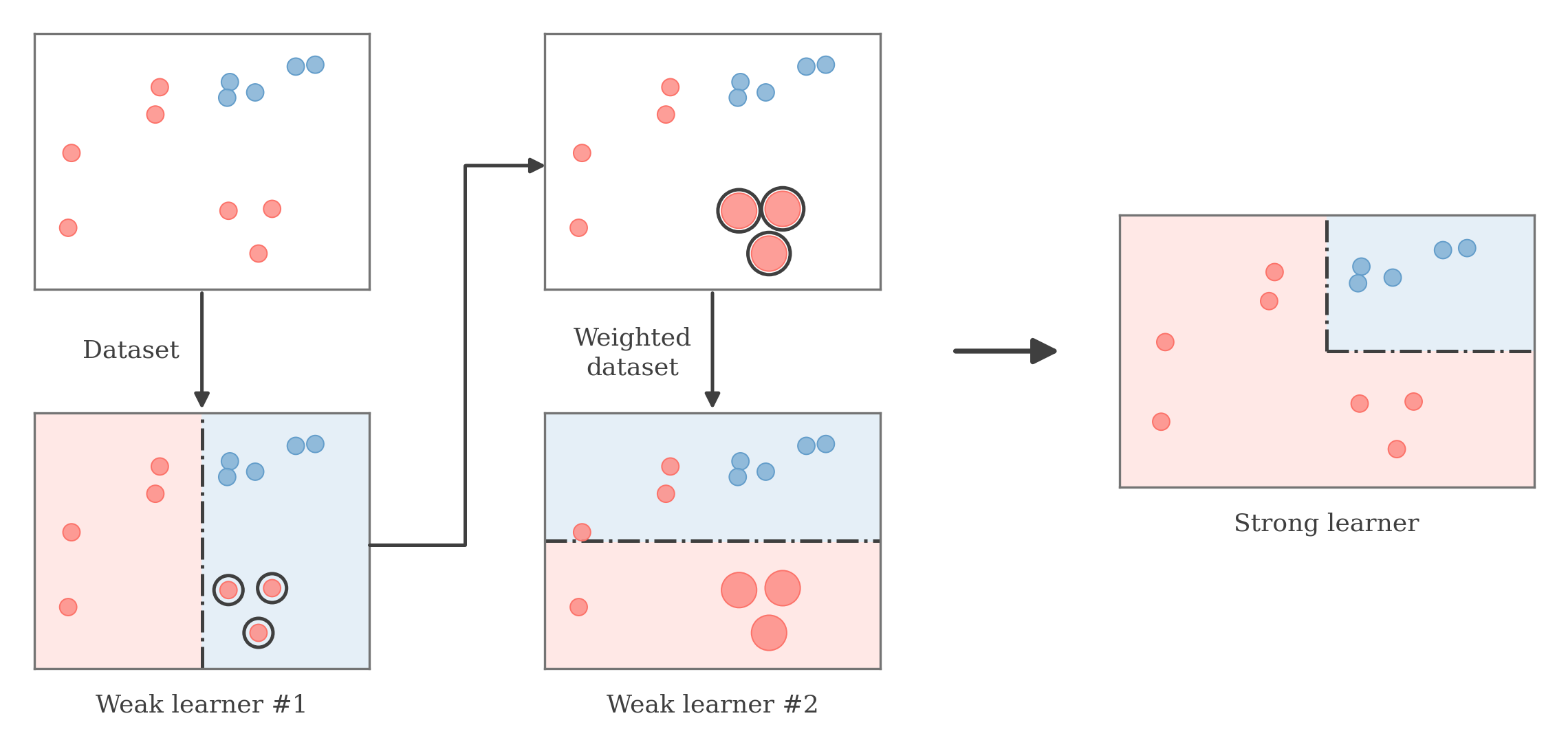
AdaBoost pipeline: dataset, weak learner, reweighted dataset, second weak learner, and the combined strong learner — Each round fits a weak learner, gives more weight to examples it misclassifies, and adds the new learner to the weighted ensemble.

We encode both the true label and each weak learner's prediction as either $-1$ or $+1$ :

y^{(i)} \in \{-1,1\}

h(x) \in \{-1,1\}

With this encoding:

y^{(i)}h(x^{(i)})=1

when the prediction is correct, and:

y^{(i)}h(x^{(i)})=-1

when it is wrong.

AdaBoost uses exponential loss:

\ell_i(H) = e^{-y^{(i)}H(x^{(i)})}

and the total training loss is:

\mathcal L(H) = \sum_{i=1}^n e^{-y^{(i)}H(x^{(i)})}

Correct predictions with a large positive margin have small loss, while incorrect predictions have large loss.

The derivative with respect to the prediction for example $i$ is:

\frac{ \partial\mathcal L }{ \partial H(x^{(i)}) } = -y^{(i)} e^{-y^{(i)}H(x^{(i)})}

This naturally gives more importance to examples with large exponential loss.

Define the normalized weight of example $i$ at round $t$ as:

w_t^{(i)} = \frac{ e^{-y^{(i)}H_t(x^{(i)})} }{ \sum_{j=1}^n e^{-y^{(j)}H_t(x^{(j)})} }

Examples that the current ensemble handles poorly receive larger weights.

The next weak learner minimizes the weighted classification error:

h_{t+1} = \arg\min_{h\in\mathcal H} \sum_{i=1}^n w_t^{(i)} 1\left\{ y^{(i)} \neq h(x^{(i)}) \right\}

See derivation

The weak learner should point against the gradient:

h_{t+1} = \arg\min_{h\in\mathcal H} \sum_{i=1}^n \frac{ \partial\mathcal L }{ \partial H(x^{(i)}) } h(x^{(i)})

Substituting the derivative of the exponential loss:

= \arg\min_{h\in\mathcal H} \left[ - \sum_{i=1}^n y^{(i)} h(x^{(i)}) e^{-y^{(i)}H_t(x^{(i)})} \right]

= \arg\min_{h\in\mathcal H} \left[ - \sum_{i=1}^n y^{(i)} h(x^{(i)}) w_t^{(i)} \right]

Because both $y^{(i)}$ and $h(x^{(i)})$ are in ${-1,1}$ :

-y^{(i)}h(x^{(i)}) = \begin{cases} -1, & y^{(i)}=h(x^{(i)}) \\ 1, & y^{(i)}\neq h(x^{(i)}) \end{cases}

Therefore:

- \sum_{i=1}^n y^{(i)} h(x^{(i)}) w_t^{(i)}

= \sum_{i=1}^n 1\left\{ y^{(i)}\neq h(x^{(i)}) \right\} w_t^{(i)} - \sum_{i=1}^n 1\left\{ y^{(i)}=h(x^{(i)}) \right\} w_t^{(i)}

= 2 \sum_{i=1}^n 1\left\{ y^{(i)}\neq h(x^{(i)}) \right\} w_t^{(i)} - 1

The constant factor $2$ and constant term $-1$ do not affect the minimizer.

Therefore:

h_{t+1} = \arg\min_{h\in\mathcal H} \sum_{i=1}^n w_t^{(i)} 1\left\{ y^{(i)}\neq h(x^{(i)}) \right\}

Let the weighted error of the selected weak learner be:

\epsilon_t = \sum_{i=1}^n w_t^{(i)} 1\left\{ y^{(i)} \neq h_t(x^{(i)}) \right\}

Once we choose the weak learner, we still need to decide how much influence it should have in the ensemble.

AdaBoost chooses the step size that minimizes the exponential loss:

\alpha_t = \arg\min_\alpha \mathcal L \left( H_{t-1} + \alpha h_t \right)

This gives:

\alpha_t = \frac12 \ln \left( \frac{1-\epsilon_t}{\epsilon_t} \right)

If:

0<\epsilon_t<\frac12

then:

\alpha_t>0

A more accurate weak learner has smaller $\epsilon_t$ and therefore receives a larger weight in the final ensemble.

If:

\epsilon_t=\frac12

then:

\alpha_t=0

so the learner contributes nothing.

See derivation

We choose:

\alpha = \arg\min_\alpha \mathcal L(H_t+\alpha h)

Using exponential loss:

\alpha = \arg\min_\alpha \sum_{i=1}^n e^{-y^{(i)} \left( H_t(x^{(i)}) + \alpha h(x^{(i)}) \right)}

Differentiate with respect to $\alpha$ and set the result equal to $0$ :

- \sum_{i=1}^n y^{(i)} h(x^{(i)}) e^{-y^{(i)}H_t(x^{(i)})} e^{-\alpha y^{(i)}h(x^{(i)})} = 0

e^{-\alpha} \sum_{i:y^{(i)}=h(x^{(i)})} e^{-y^{(i)}H_t(x^{(i)})} = e^\alpha \sum_{i:y^{(i)}\neq h(x^{(i)})} e^{-y^{(i)}H_t(x^{(i)})}

Divide by the normalization constant used to define $w^{(i)}$ :

e^{-\alpha} \sum_{i:y^{(i)}=h(x^{(i)})} w^{(i)} = e^\alpha \sum_{i:y^{(i)}\neq h(x^{(i)})} w^{(i)}

The total weight of the incorrectly classified examples is:

\epsilon = \sum_{i:y^{(i)}\neq h(x^{(i)})} w^{(i)}

so the total weight of the correctly classified examples is:

1-\epsilon

Therefore:

e^{-\alpha}(1-\epsilon) = e^\alpha\epsilon

e^{2\alpha} = \frac{1-\epsilon}{\epsilon}

Taking logs:

2\alpha = \ln \left( \frac{1-\epsilon}{\epsilon} \right)

Therefore:

\alpha = \frac12 \ln \left( \frac{1-\epsilon}{\epsilon} \right)

After adding the weak learner, AdaBoost changes the example weights.

Misclassified examples receive more weight, while correctly classified examples receive less.

Before normalization:

w_{t+1}^{(i)} \propto w_t^{(i)} e^{-\alpha_t y^{(i)}h_t(x^{(i)})}

Because:

y^{(i)}h_t(x^{(i)}) = 1

for a correct prediction, its weight is multiplied by:

e^{-\alpha_t}

For a misclassified example:

y^{(i)}h_t(x^{(i)}) = -1

so its weight is multiplied by:

e^{\alpha_t}

We then normalize the weights so they sum to $1$ :

w_{t+1}^{(i)} = \frac{ w_t^{(i)} e^{-\alpha_t y^{(i)}h_t(x^{(i)})} }{ \sum_{j=1}^n w_t^{(j)} e^{-\alpha_t y^{(j)}h_t(x^{(j)})} }

For the optimal AdaBoost step size, the normalization factor has a closed form.

See derivation

Let:

Z_t = \sum_{i=1}^n w_t^{(i)} e^{-\alpha_t y^{(i)}h_t(x^{(i)})}

Split the sum into correctly and incorrectly classified examples:

Z_t = e^{-\alpha_t}(1-\epsilon_t) + e^{\alpha_t}\epsilon_t

Using:

\alpha_t = \frac12 \ln \left( \frac{1-\epsilon_t}{\epsilon_t} \right)

we have:

e^{-\alpha_t} = \sqrt{ \frac{\epsilon_t}{1-\epsilon_t} }

and:

e^{\alpha_t} = \sqrt{ \frac{1-\epsilon_t}{\epsilon_t} }

Therefore:

Z_t = \sqrt{ \frac{\epsilon_t}{1-\epsilon_t} } (1-\epsilon_t) + \sqrt{ \frac{1-\epsilon_t}{\epsilon_t} } \epsilon_t

= 2 \sqrt{ \epsilon_t(1-\epsilon_t) }

After $T$ rounds, the ensemble is:

H_T(x) = \sum_{t=1}^T \alpha_t h_t(x)

AdaBoost predicts using the sign of this weighted vote:

\widehat y(x) = \operatorname{sign} \left( H_T(x) \right)

= \operatorname{sign} \left( \sum_{t=1}^T \alpha_t h_t(x) \right)

The standard closed-form step assumes:

0<\epsilon_t<\frac12

If $\epsilon_t=0$ , the weak learner perfectly classifies all examples with positive weight, so boosting can stop.

If $\epsilon_t\geq\frac12$ , the learner has no positive edge under the current weights and should not be added in this form.

H\leftarrow0

\text{For each }i,\quad w^{(i)} \leftarrow \frac1n

\text{Repeat } \{

\quad h \leftarrow \arg\min_{h\in\mathcal H} \sum_{i=1}^n w^{(i)} 1\left\{ y^{(i)} \neq h(x^{(i)}) \right\}

\quad \epsilon \leftarrow \sum_{i=1}^n w^{(i)} 1\left\{ y^{(i)} \neq h(x^{(i)}) \right\}

\quad \alpha \leftarrow \frac12 \ln \left( \frac{1-\epsilon}{\epsilon} \right)

\quad H \leftarrow H+\alpha h

\quad \text{For each }i,\quad w^{(i)} \leftarrow w^{(i)} e^{-\alpha y^{(i)}h(x^{(i)})}

\quad \text{Normalize the weights so that } \sum_i w^{(i)}=1

\}