Learning Theory and Generalization

Bias-Variance Tradeoff

Why can two models with similar training error behave very differently on new data?

One way to understand this is through the bias-variance decomposition. For squared-error regression, prediction error can be separated into three parts: noise, bias, and variance.

We first look at the error for a single input $x$ .

Write the response as:

Y = f^*(x) + \xi

where:

f^*(x) = \mathbb E[Y\mid X=x]

is the best possible prediction under squared error, and $\xi$ represents the remaining noise:

\mathbb E[\xi\mid X=x] = 0

\operatorname{Var}(\xi\mid X=x) = \sigma^2(x)

The noise does not need to be Gaussian.

Now imagine repeatedly drawing a new training set and fitting the same learning algorithm each time.

Let $S$ denote one such training set, and let $h_S$ be the model learned from it.

Because the training data changes, the learned prediction:

h_S(x)

can also change.

We measure the expected squared error on a fresh test response at the same input $x$ :

\mathbb E_{S,Y\mid x} \left[ \left( Y-h_S(x) \right)^2 \right]

If we average the prediction over all possible training sets, we get:

h_{\mathrm{avg}}(x) = \mathbb E_S[h_S(x)]

This tells us what the learning algorithm predicts on average.

The expected error can then be decomposed as:

\mathbb E_{S,Y\mid x} \left[ \left( Y-h_S(x) \right)^2 \right]

= \sigma^2(x) + \underbrace{ \left( f^*(x)-h_{\mathrm{avg}}(x) \right)^2 }_{\text{bias}^2} + \underbrace{ \operatorname{Var}_S \left( h_S(x) \right) }_{\text{variance}}

The three terms have different meanings.

The noise term:

\sigma^2(x)

is unavoidable. Even the optimal predictor $f^*(x)$ cannot predict the random noise in $Y$ .

The squared bias:

\left( f^*(x)-h_{\mathrm{avg}}(x) \right)^2

measures how far the model's average prediction is from the optimal prediction.

Large bias means the model makes a systematic error and is often associated with underfitting.

The variance:

\operatorname{Var}_S \left( h_S(x) \right)

measures how much the model's prediction changes when we train it on a different dataset.

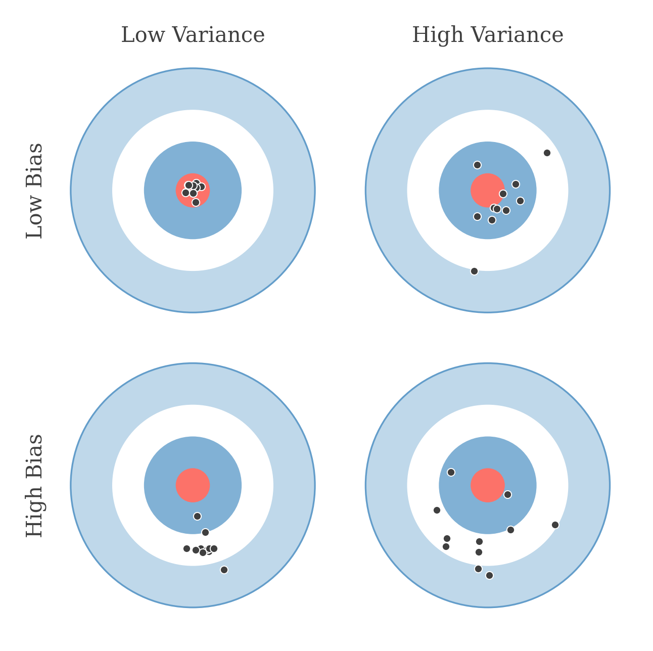
Bias-variance bullseye: four targets showing low and high bias against low and high variance — Each shot represents a model trained on a different dataset. Bias measures how far the average prediction is from the target, while variance measures how spread out the predictions are.

Averaging the pointwise decomposition over the distribution of $X$ gives the overall test mean squared error.

See derivation

Substitute:

Y = f^*(x) + \xi

into the expected squared error:

\mathbb E \left[ \left( Y-h_S(x) \right)^2 \right]

= \mathbb E \left[ \left( f^*(x) + \xi - h_S(x) \right)^2 \right]

= \mathbb E \left[ \left( \xi + f^*(x) - h_S(x) \right)^2 \right]

= \mathbb E[\xi^2] + \mathbb E \left[ \left( f^*(x)-h_S(x) \right)^2 \right]

= \sigma^2(x) + \mathbb E \left[ \left( f^*(x)-h_S(x) \right)^2 \right]

Now add and subtract $h_{\mathrm{avg}}(x)$ :

= \sigma^2(x) + \mathbb E \left[ \left( f^*(x) - h_{\mathrm{avg}}(x) + h_{\mathrm{avg}}(x) - h_S(x) \right)^2 \right]

Expanding the square gives:

= \sigma^2(x) + \left( f^*(x)-h_{\mathrm{avg}}(x) \right)^2

+ \mathbb E_S \left[ \left( h_{\mathrm{avg}}(x)-h_S(x) \right)^2 \right]

+ 2 \left( f^*(x)-h_{\mathrm{avg}}(x) \right) \mathbb E_S \left[ h_{\mathrm{avg}}(x)-h_S(x) \right]

\mathbb E_S \left[ h_{\mathrm{avg}}(x)-h_S(x) \right] = 0

Therefore:

= \sigma^2(x) + \left( f^*(x)-h_{\mathrm{avg}}(x) \right)^2 + \mathbb E_S \left[ \left( h_{\mathrm{avg}}(x)-h_S(x) \right)^2 \right]

\mathbb E_S \left[ \left( h_{\mathrm{avg}}(x)-h_S(x) \right)^2 \right] = \operatorname{Var}_S \left( h_S(x) \right)

So:

\mathbb E_{S,Y\mid x} \left[ \left( Y-h_S(x) \right)^2 \right]

= \sigma^2(x) + \left( f^*(x)-h_{\mathrm{avg}}(x) \right)^2 + \operatorname{Var}_S \left( h_S(x) \right)

Model Capacity and Double Descent

As model capacity increases, a classical pattern is:

bias tends to decrease because the model can represent more complex relationships;
variance can increase because the learned model becomes more sensitive to the training data.

This can produce a U-shaped test-error curve.

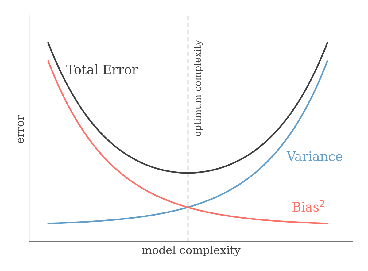
Bias-variance tradeoff: bias squared falling and variance rising, summing to a U-shaped total error — In the classical picture, squared bias decreases as model capacity grows while variance increases, producing an intermediate minimum in test error.

This is a useful heuristic, not a universal law.

Model capacity is also more subtle than simply counting parameters.

Some modern models exhibit double descent.

Instead of following a single U-shaped curve, test error can first decrease, then rise near the point where the model can perfectly fit the training data, and then decrease again as capacity increases further.

The point where the model first reaches zero training error is called the interpolation threshold.

For squared-error regression, interpolation means:

h(x^{(i)}) = y^{(i)}

for every training example.

For classification, it often means zero training classification error.

Near the interpolation threshold, fitting the training data exactly can make the learned solution especially sensitive to small changes in the dataset.

The location of this threshold depends on the model, data, regularization, and optimization.

It is not generally the simple condition that the number of parameters equals the number of training examples.

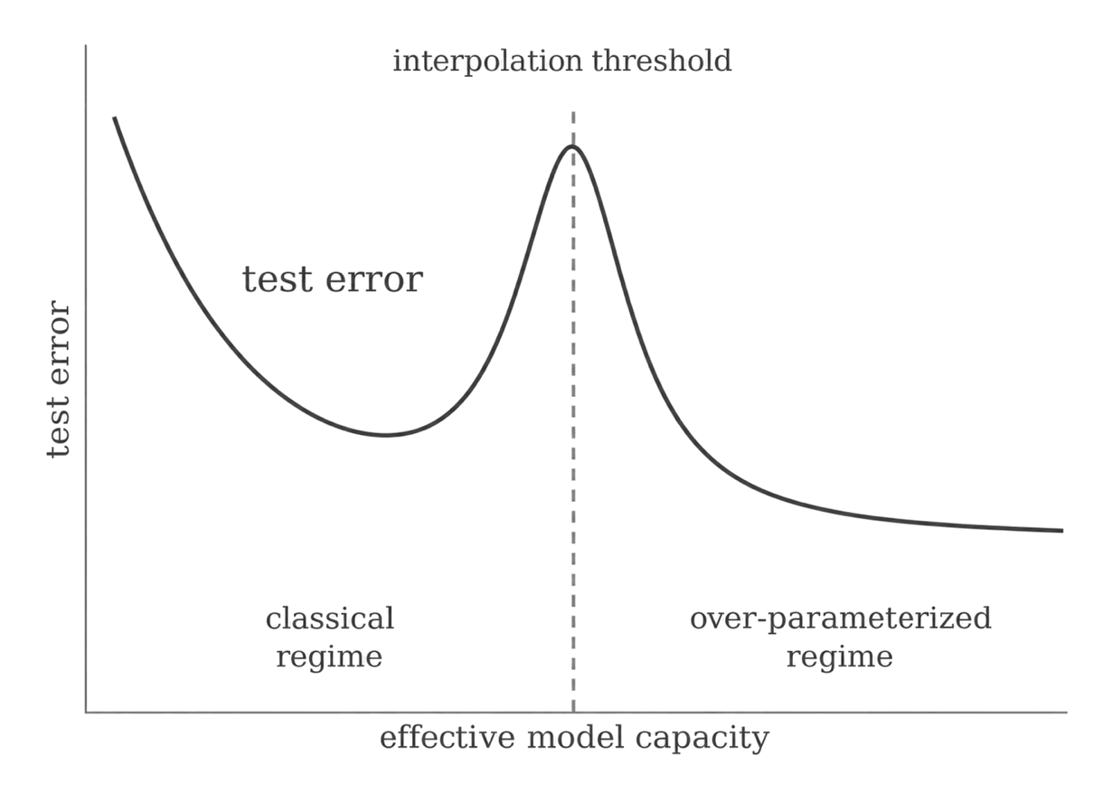
Double descent curve: test error peaks at the interpolation threshold then descends again — In a schematic double-descent curve, test error rises near the interpolation threshold and then falls again as effective model capacity continues to increase.

Complexity Bounds

Training error tells us how well a model fits the examples we observed.

What we really care about, however, is how well it performs on new examples.

Complexity bounds give us a way to relate these two quantities.

Let:

S = \{(X_i,Y_i)\}_{i=1}^n

be a training sample drawn IID from an unknown distribution $\mathcal D$ .

For a classifier $h$ , the population error is the probability that it misclassifies a fresh example drawn from $\mathcal D$ :

\epsilon(h) = P_{(X,Y)\sim\mathcal D} \left( h(X)\neq Y \right)

We do not know the true distribution $\mathcal D$ , so we usually cannot compute this quantity directly.

Instead, we measure the fraction of mistakes on the training sample.

This is the empirical error:

\widehat\epsilon_S(h) = \frac1n \sum_{i=1}^n 1 \left\{ h(X_i)\neq Y_i \right\}

A natural strategy is to choose the hypothesis with the smallest empirical error.

This is called empirical risk minimization, or ERM.

Let $\mathcal H$ be a finite hypothesis class with:

|\mathcal H| = K

Then ERM selects:

\widehat h \in \arg\min_{h\in\mathcal H} \widehat\epsilon_S(h)

But a model with low training error does not necessarily have low population error.

We therefore want to understand the gap:

\left| \epsilon(h) - \widehat\epsilon_S(h) \right|

between population and empirical performance.

Hoeffding Inequality

Hoeffding's inequality tells us how quickly an empirical average concentrates around its true mean.

Imagine a coin that lands heads with probability $\phi$ .

Let:

Z_1,\ldots,Z_n

be independent Bernoulli random variables representing the coin tosses, and let:

\widehat\phi = \frac1n \sum_{i=1}^n Z_i

be the observed fraction of heads.

Hoeffding's inequality states that for any $\gamma>0$ :

P \left( \left| \phi-\widehat\phi \right| > \gamma \right) \leq 2 \exp \left( -2\gamma^2 n \right)

As $n$ grows, the probability of a large difference between the empirical frequency and the true probability decreases exponentially.

Uniform Convergence

For one fixed classifier $h$ , Hoeffding's inequality immediately gives a bound on the gap between training error and population error.

Define:

Z_i(h) = 1 \left\{ h(X_i)\neq Y_i \right\}

Then:

P_S \left( \left| \epsilon(h) - \widehat\epsilon_S(h) \right| > \gamma \right) \leq 2 \exp \left( -2\gamma^2n \right)

But this is not enough for ERM.

The classifier:

\widehat h

is chosen after looking at the training data.

To handle this data-dependent choice, we want the bound to hold for every hypothesis in $\mathcal H$ at the same time.

For a finite class containing $K$ hypotheses, we can do this with the union bound.

The result is:

P_S \left( \forall h\in\mathcal H: \left| \epsilon(h) - \widehat\epsilon_S(h) \right| \leq \gamma \right) \geq 1 - 2K \exp \left( -2\gamma^2n \right)

This is called a uniform convergence bound.

It shows two important effects.

More training examples make the guarantee tighter.

A larger hypothesis class makes the guarantee weaker.

The intuition is that with more possible hypotheses, there are more chances for at least one model to look unusually good on the training sample.

This does not mean that a larger hypothesis class has worse training error.

A larger class can only improve or preserve the best achievable empirical error.

The bound concerns the gap between training and population performance.

Because the guarantee holds for every hypothesis on the same event, it also applies to the data-dependent ERM solution $\widehat h$ .

See derivation

For events:

A_1,\ldots,A_K

the union bound gives:

P \left( A_1\cup\cdots\cup A_K \right) \leq \sum_{j=1}^K P(A_j)

Enumerate:

\mathcal H = \{h_1,\ldots,h_K\}

and define the bad event:

A_j = \left\{ \left| \epsilon(h_j) - \widehat\epsilon_S(h_j) \right| > \gamma \right\}

Hoeffding's inequality gives:

P_S(A_j) \leq 2 \exp \left( -2\gamma^2n \right)

Therefore:

P_S \left( \exists h\in\mathcal H: \left| \epsilon(h) - \widehat\epsilon_S(h) \right| > \gamma \right)

= P_S \left( A_1\cup\cdots\cup A_K \right)

\leq \sum_{j=1}^K P_S(A_j)

\leq 2K \exp \left( -2\gamma^2n \right)

P_S \left( \forall h\in\mathcal H: \left| \epsilon(h) - \widehat\epsilon_S(h) \right| \leq \gamma \right) \geq 1 - 2K \exp \left( -2\gamma^2n \right)

Sample Complexity

We can now ask:

How many training examples are sufficient to guarantee a generalization gap of at most $\gamma$ with probability at least $1-\delta$ ?

We want the failure probability to be at most:

\delta

so we require:

2K \exp \left( -2\gamma^2n \right) \leq \delta

Solving for $n$ gives:

n \geq \frac{1}{2\gamma^2} \log \frac{2K}{\delta}

This is a sample-complexity bound.

It shows that:

requiring a smaller error tolerance $\gamma$ needs substantially more data because of the $1/\gamma^2$ dependence;
allowing a larger hypothesis class increases the requirement through $\log K$ ;
demanding higher confidence increases the requirement through $\log(1/\delta)$ .

Equivalently, if the sample size $n$ is fixed, the same result tells us how large the generalization gap can be.

With probability at least $1-\delta$ :

\forall h\in\mathcal H: \qquad \left| \epsilon(h) - \widehat\epsilon_S(h) \right| \leq \sqrt{ \frac{1}{2n} \log \frac{2K}{\delta} }

This is a high-probability statement.

It does not say that the gap is deterministically below this value for every possible training sample.

See derivation

Starting from:

2K e^{-2\gamma^2n} \leq \delta

-2\gamma^2n \leq \log \frac{\delta}{2K}

Multiplying by $-1$ reverses the inequality:

2\gamma^2n \geq \log \frac{2K}{\delta}

Therefore:

\gamma^2 \geq \frac{1}{2n} \log \frac{2K}{\delta}

and:

\gamma \geq \sqrt{ \frac{1}{2n} \log \frac{2K}{\delta} }

Choosing the right-hand side as the deviation threshold gives the uniform guarantee with probability at least $1-\delta$ .

ERM Generalization Guarantee

Uniform convergence lets us say something stronger about the model selected by ERM.

Let:

h_{\mathcal H}^* \in \arg\min_{h\in\mathcal H} \epsilon(h)

be the hypothesis in $\mathcal H$ with the smallest population error.

Also define:

\gamma_\delta = \sqrt{ \frac{1}{2n} \log \frac{2K}{\delta} }

On the uniform-convergence event:

\epsilon(\widehat h) \leq \epsilon \left( h_{\mathcal H}^* \right) + 2\gamma_\delta

or:

\epsilon(\widehat h) \leq \epsilon \left( h_{\mathcal H}^* \right) + 2 \sqrt{ \frac{1}{2n} \log \frac{2K}{\delta} }

So ERM performs nearly as well as the best hypothesis available in $\mathcal H$ , provided empirical and population errors are uniformly close.

This guarantee holds with probability at least $1-\delta$ over the random draw of the training set.

It does not hold for every possible sample.

See derivation

On the event that:

\left| \epsilon(h) - \widehat\epsilon_S(h) \right| \leq \gamma_\delta

for every $h\in\mathcal H$ :

\epsilon(\widehat h) \leq \widehat\epsilon_S(\widehat h) + \gamma_\delta

\widehat\epsilon_S(\widehat h) \leq \widehat\epsilon_S \left( h_{\mathcal H}^* \right)

Therefore:

\epsilon(\widehat h) \leq \widehat\epsilon_S \left( h_{\mathcal H}^* \right) + \gamma_\delta

Using uniform convergence again:

\widehat\epsilon_S \left( h_{\mathcal H}^* \right) \leq \epsilon \left( h_{\mathcal H}^* \right) + \gamma_\delta

so:

\epsilon(\widehat h) \leq \epsilon \left( h_{\mathcal H}^* \right) + 2\gamma_\delta

This bound separates two sources of error.

The first term:

\epsilon \left( h_{\mathcal H}^* \right)

is the error of the best model available in the hypothesis class.

If $\mathcal H$ is too restrictive, this error can be large.

This is related to approximation error.

The second term:

2 \sqrt{ \frac{1}{2n} \log \frac{2K}{\delta} }

is an estimation or complexity term.

It reflects the difficulty of choosing a good hypothesis from a finite amount of data.

Enlarging $\mathcal H$ can reduce approximation error because more models become available.

However, it can increase this particular complexity bound through $\log K$ .

This resembles the bias-variance tradeoff, but the two ideas are not mathematically identical.