Unsupervised Learning and Representation

K-means

Sometimes we have data without labels and want to discover groups within it. This is called clustering.

K-means is a clustering algorithm that groups nearby points together. Each group is represented by a point called a centroid.

K-means alternates between two simple steps:

assign every point to its nearest centroid;
move each centroid to the mean of the points assigned to it.

We use $c^{(i)}$ for the cluster assigned to example $x^{(i)}$ , and $\mu_j$ for the centroid of cluster $j$ .

\text{Initialize cluster centroids } \mu_1,\ldots,\mu_k

\text{Repeat until convergence } \{

\quad \text{For each }i,\quad c^{(i)} \leftarrow \arg\min_j \left\| x^{(i)}-\mu_j \right\|_2^2

\quad \text{For each }j,\quad \mu_j \leftarrow \frac{ \sum_{i=1}^n 1\left\{ c^{(i)}=j \right\} x^{(i)} }{ \sum_{i=1}^n 1\left\{ c^{(i)}=j \right\} }

\}

The first step assigns each point to its nearest centroid.

The second step moves each centroid to the mean of the points assigned to it.

We repeat these steps until the assignments stop changing, or until the centroids move by only a very small amount.

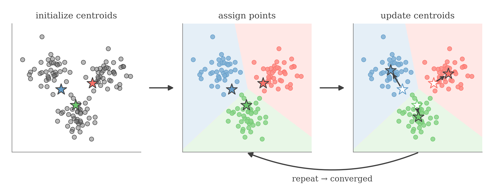
Three panels showing one round of k-means: randomly placed initial centroids, points assigned to their nearest centroid with the resulting Voronoi regions, then each centroid moved to the mean of its assigned points — K-means alternates between assigning points to their nearest centroid and moving each centroid to the mean of its assigned points.

A practical issue occurs if a cluster receives no points. Its mean is then undefined, so an implementation must keep or reinitialize that centroid before continuing.

K-means tries to keep every point close to its assigned centroid.

Its objective, called the distortion, is:

J(c,\mu) = \sum_{i=1}^n \left\| x^{(i)} - \mu_{c^{(i)}} \right\|_2^2

Smaller $J$ means the clusters are more compact.

Each assignment step and centroid-update step can only decrease $J$ or leave it unchanged.

K-means therefore eventually reaches a solution where the assignments stop changing.

However, this solution may only be a local minimum.

Different initial centroids can produce different final clusters.

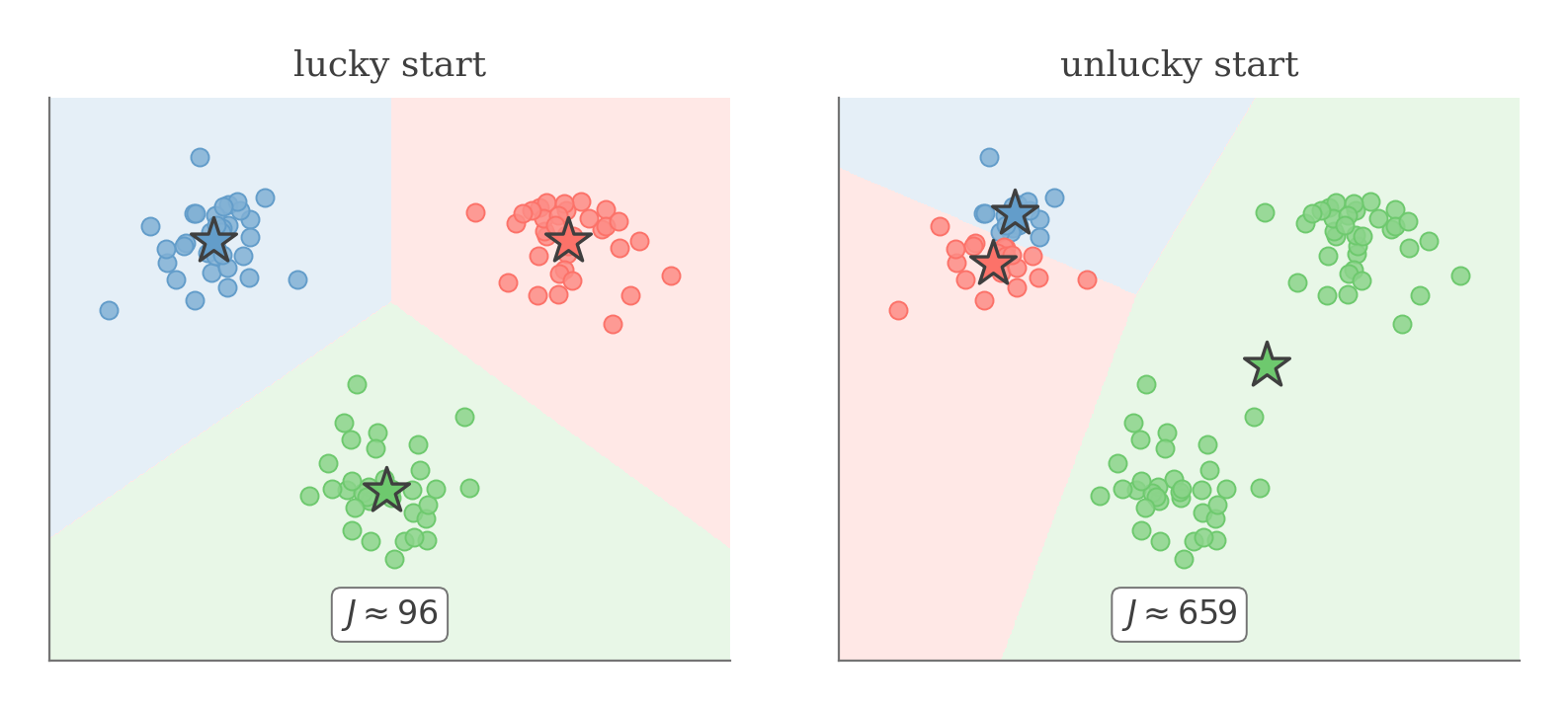
The same dataset clustered two ways: a good initialization recovers the three clusters at low distortion, while a bad initialization splits one cluster between two centroids and merges the other two, giving a much higher distortion — Different initial centroids can lead to very different solutions. In practice, we run K-means several times and keep the solution with the smallest distortion.

For this reason, we usually run K-means several times with different initial centroids and keep the solution with the smallest $J$ .

Because K-means uses squared Euclidean distance, feature scaling matters. A feature with a much larger numerical scale can dominate the distance calculation.

K-means also works best when clusters are reasonably compact and roughly spherical. It can perform poorly for elongated clusters, clusters with very different densities, or categorical features.

The number of clusters $k$ must also be chosen separately.

Principal Component Analysis

Principal Component Analysis, or PCA, finds directions along which the data varies the most.

We can use these directions to represent high-dimensional data using fewer dimensions while preserving as much variation as possible.

Before applying ordinary PCA, we center the data so that each feature has mean zero.

For feature $j$ , compute its mean:

\mu_j = \frac{1}{n} \sum_{i=1}^n x_j^{(i)}

Then center the feature:

\widetilde{x}_j^{(i)} = x_j^{(i)} - \mu_j

If feature scales should not influence PCA, we can additionally standardize each feature.

Define:

\sigma_j^2 = \frac{1}{n} \sum_{i=1}^n \left( x_j^{(i)}-\mu_j \right)^2

Then:

\widehat{x}_j^{(i)} = \frac{ x_j^{(i)}-\mu_j }{ \sigma_j }

A constant feature has zero variance and cannot be standardized.

Below, $x^{(i)}$ refers to the centered data, or standardized data if we choose to standardize.

Maximum-Variance Directions

The first principal component is the direction along which the projected data has the largest variance.

Let $u$ be a unit vector representing a direction.

We want to choose the direction for which the projected points are spread out the most.

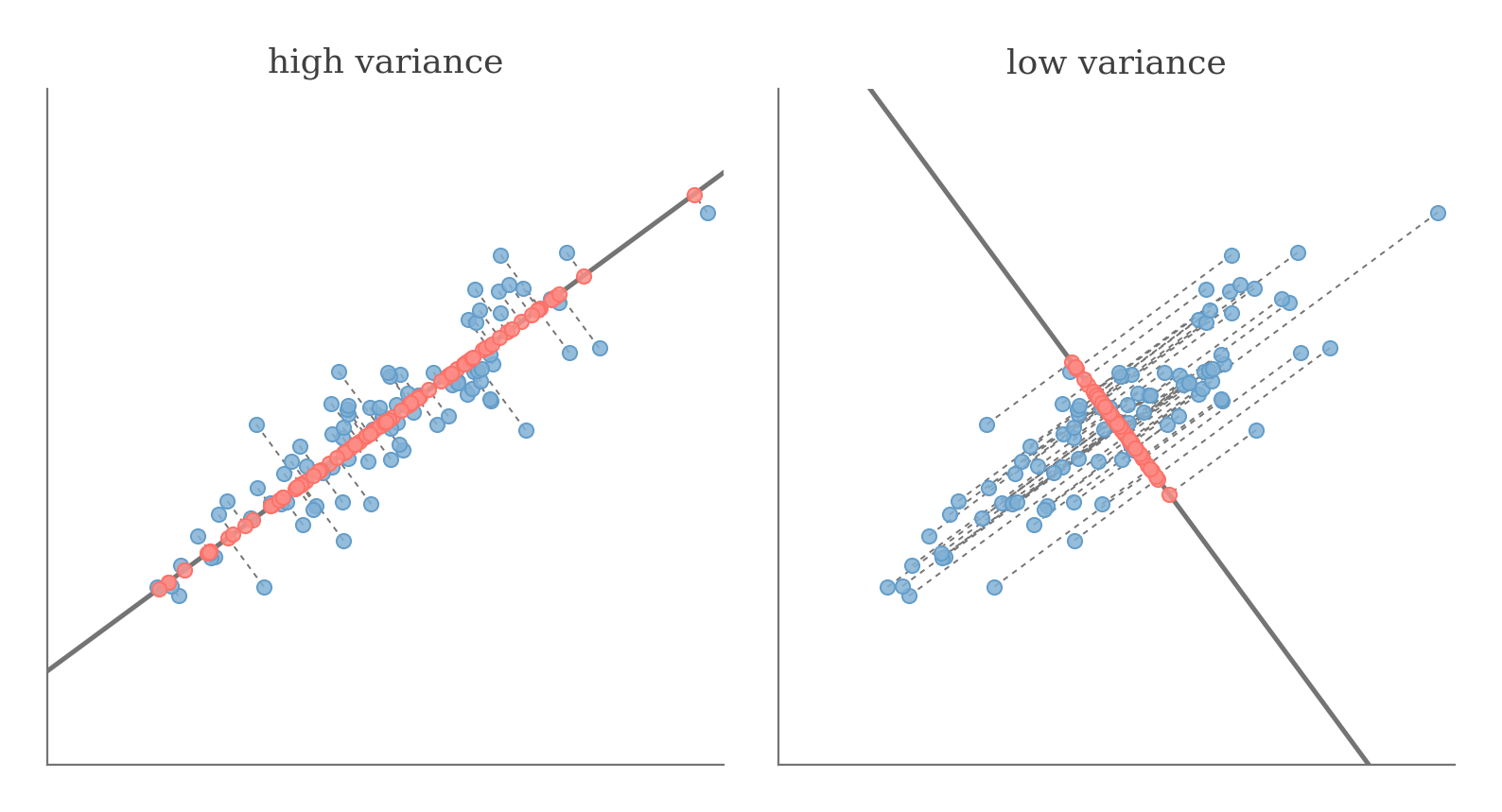
The same data projected onto a high-variance direction versus a low-variance direction — PCA chooses directions along which the projected data is as spread out as possible.

For a unit vector $u$ , the coordinate of a point $x$ along this direction is:

u^Tx

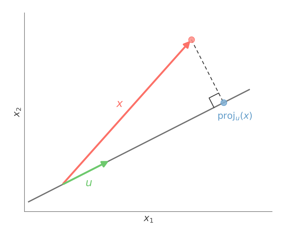
Orthogonal projection of a point x onto the unit vector u — The scalar $u^Tx$ tells us how far the point lies along the direction $u$ .

The variance of the projected data is therefore proportional to:

\frac{1}{n} \sum_{i=1}^n \left( u^Tx^{(i)} \right)^2

So the first principal component is:

u_1 = \arg\max_{\|u\|_2=1} \frac{1}{n} \sum_{i=1}^n \left( u^Tx^{(i)} \right)^2

This objective can be written using the covariance matrix.

See derivation

\frac{1}{n} \sum_{i=1}^n \left( u^Tx^{(i)} \right)^2

= \frac{1}{n} \sum_{i=1}^n u^Tx^{(i)} x^{(i)T}u

= u^T \left( \frac{1}{n} \sum_{i=1}^n x^{(i)}x^{(i)T} \right) u

Define:

\Sigma = \frac{1}{n} \sum_{i=1}^n x^{(i)}x^{(i)T}

Therefore:

u_1 = \arg\max_{\|u\|_2=1} u^T\Sigma u

Because the data has been centered, $\Sigma$ is the sample covariance matrix under this $1/n$ convention.

We now need to find the unit vector $u$ that maximizes:

u^T\Sigma u

subject to:

u^Tu=1

Using Lagrange optimization gives an eigenvalue problem.

See derivation

Define the Lagrangian:

L(u,\lambda) = u^T\Sigma u - \lambda \left( u^Tu-1 \right)

Differentiate with respect to $u$ :

\nabla_u L = 2\Sigma u - 2\lambda u

Setting the derivative equal to $0$ gives:

2\Sigma u - 2\lambda u = 0

Therefore:

\Sigma u = \lambda u

So every stationary direction is an eigenvector of the covariance matrix $\Sigma$ .

For an eigenvector $u$ , the corresponding eigenvalue $\lambda$ is the variance of the data along that direction:

u^T\Sigma u = u^T(\lambda u) = \lambda

because:

u^Tu=1

The stationary directions are eigenvectors, but we still need to determine which eigenvector gives the largest variance.

Let:

v_1,\ldots,v_d

be an orthonormal eigenbasis of $\Sigma$ , with eigenvalues:

\lambda_1 \geq \lambda_2 \geq \cdots \geq \lambda_d \geq 0

See derivation

Any unit vector can be written as:

u = \sum_{j=1}^d a_jv_j

where:

\sum_{j=1}^d a_j^2 = 1

Then:

u^T\Sigma u

= \sum_{j=1}^d \lambda_j a_j^2

\leq \lambda_1 \sum_{j=1}^d a_j^2

= \lambda_1

Therefore, the variance is maximized by an eigenvector corresponding to the largest eigenvalue.

The first principal component is:

u_1=v_1

The second principal component is the orthogonal direction with the next largest variance:

u_2=v_2

and so on.

If the largest eigenvalue is repeated, any unit vector in its eigenspace is optimal.

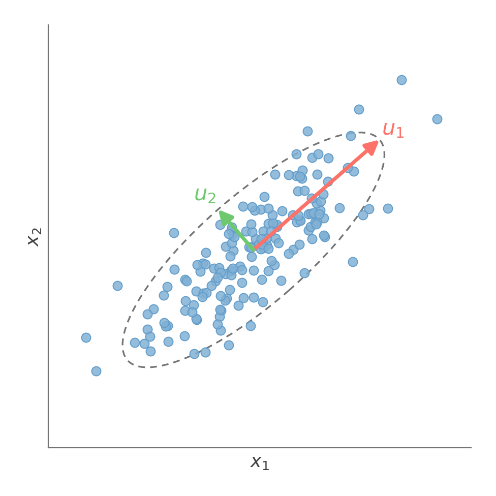
Data cloud with the two principal component directions drawn as arrows from the center — The principal components are eigenvectors of the covariance matrix. The first points in the direction of greatest variance, while later components capture the largest remaining orthogonal directions of variation.

If we want to reduce the data to $k$ dimensions, we keep the top $k$ principal components:

U_k = \begin{bmatrix} u_1 & u_2 & \cdots & u_k \end{bmatrix}

A centered point $x\in\mathbb R^d$ is then represented by:

z = U_k^Tx

where:

z\in\mathbb R^k

is the lower-dimensional representation of $x$ .

In practice, we choose the eigenvectors corresponding to the largest eigenvalues.

These can be computed from an eigendecomposition of the covariance matrix or directly from the centered data using singular value decomposition.

Independent Component Analysis

Independent Component Analysis, or ICA, tries to recover independent signals that have been mixed together.

A classic example is the cocktail party problem: several people speak at the same time, and several microphones record different mixtures of their voices.

We represent the original sources by:

s\in\mathbb R^d

and the observed mixtures by:

x\in\mathbb R^d

The mixing process is:

x = As

where:

A\in\mathbb R^{d\times d}

is the mixing matrix.

The matrix $A$ tells us how much of each source appears in each observed signal.

ICA tries to reverse this mixing.

After centering the observations, ICA learns an unmixing matrix $W$ such that:

\widehat s = Wx

If the model is correct:

W \approx A^{-1}

and the recovered coordinates $\widehat s_j$ are as statistically independent as possible.

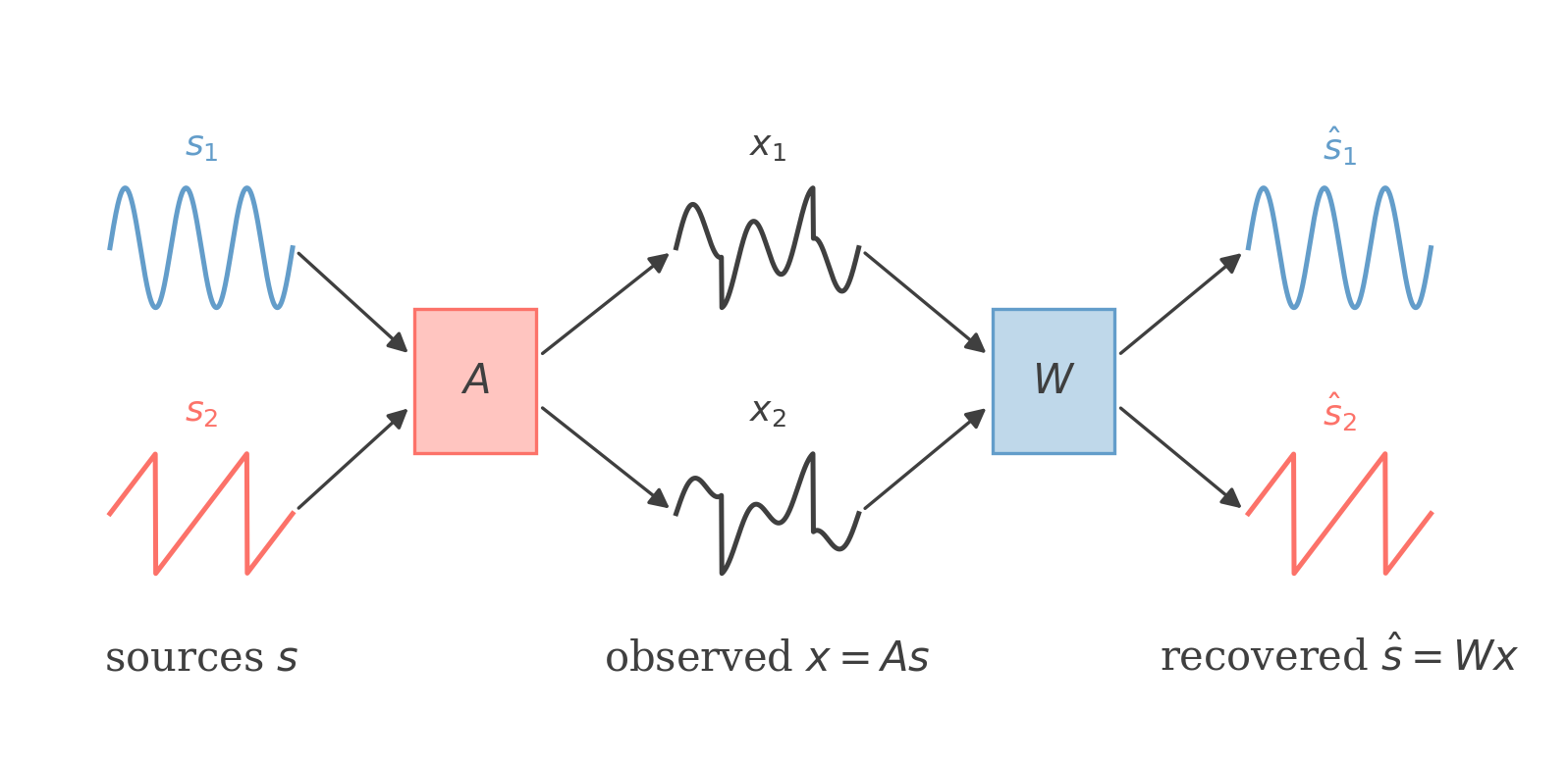
Independent sources mixed into observed microphone signals, then unmixed to recover the sources — Several independent sources are mixed into the observed signals. ICA learns a transformation that tries to separate those mixtures back into the original sources.

The key assumption is that the original sources are statistically independent.

If source $s_j$ has density $p_{s_j}$ , independence means that the joint density factorizes:

p_s(s) = \prod_{j=1}^d p_{s_j}(s_j)

So knowing one source does not provide information about the value of another.

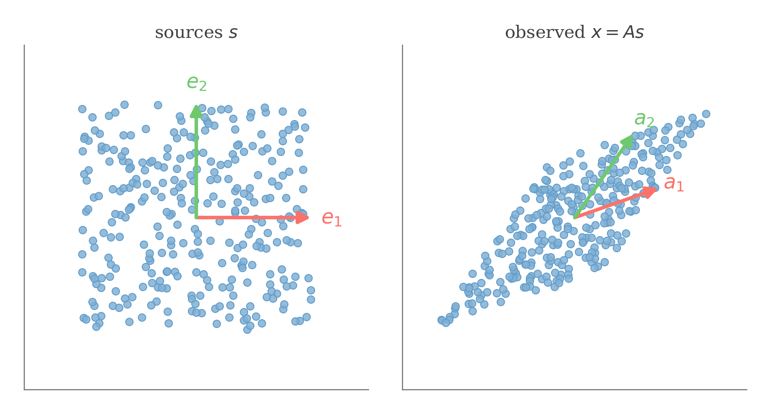
Independent sources forming a square sheared by the mixing matrix into a parallelogram — Mixing transforms the independent source coordinates into new directions. ICA tries to recover the directions that make the transformed coordinates independent again.

Likelihood and Learning

To learn $W$ using likelihood, we need the probability density of the observed mixture $x$ .

Since:

s = Wx

we can use the change-of-variables formula.

Change of Variables in Probability

For an invertible transformation:

s = Wx

the density transforms as:

p_x(x) = p_s(Wx) |\det W|

The determinant term accounts for how the transformation $W$ expands or contracts volume.

Using the factorized source density:

p_s(s) = \prod_{j=1}^d p_{s_j}(s_j)

the likelihood of one observation becomes:

p_x(x;W) = \left( \prod_{j=1}^d p_{s_j} \left( w_j^Tx \right) \right) |\det W|

where $w_j^T$ is row $j$ of $W$ .

ICA needs a model for the distribution of each source.

One simple non-Gaussian choice is the logistic distribution, whose CDF is:

g(u) = \frac{1}{ 1+\exp(-u) }

and whose density is:

p_{s_j}(u) = g'(u)

We now choose $W$ so that the recovered coordinates are likely under these independent source distributions.

For centered observations:

x^{(1)},\ldots,x^{(n)}

the log-likelihood is:

\ell(W) = \sum_{i=1}^n \sum_{j=1}^d \log g' \left( w_j^Tx^{(i)} \right) + n\log|\det W|

The first term rewards recovered coordinates that look like samples from the assumed source distributions.

The log-determinant term comes from the change of variables and accounts for how the transformation changes volume.

To write the gradient compactly, define the recovered source vector:

u^{(i)} = Wx^{(i)}

and define:

\varphi(u) = \begin{pmatrix} 1-2g(u_1) \\ \vdots \\ 1-2g(u_d) \end{pmatrix}

Each component of $\varphi(u)$ is the derivative of $\log g'(u_j)$ with respect to $u_j$ .

Differentiating the likelihood gives the gradient.

See derivation

The sigmoid satisfies:

g'(u) = g(u) \left( 1-g(u) \right)

For one recovered coordinate:

\frac{d}{du} \log g'(u)

= \frac{d}{du} \left[ \log g(u) + \log \left( 1-g(u) \right) \right]

= \frac{g'(u)}{g(u)} - \frac{g'(u)}{1-g(u)}

= 1-g(u)-g(u)

= 1-2g(u)

Therefore, the source-density terms contribute:

\sum_{i=1}^n \varphi \left( Wx^{(i)} \right) x^{(i)T}

For the determinant term:

\nabla_W \log|\det W| = W^{-T}

Because the log-determinant appears once for each of the $n$ observations, its contribution is:

nW^{-T}

Therefore:

\nabla_W\ell(W) = \sum_{i=1}^n \varphi \left( Wx^{(i)} \right) x^{(i)T} + nW^{-T}

The batch gradient-ascent update is therefore:

W \leftarrow W + \alpha \nabla_W\ell(W)

or:

W \leftarrow W + \alpha \left[ \sum_{i=1}^n \varphi \left( Wx^{(i)} \right) x^{(i)T} + nW^{-T} \right]

Instead of using all $n$ examples in every update, we can update $W$ using one example at a time.

For stochastic gradient ascent:

W \leftarrow W + \alpha \left[ \varphi \left( Wx^{(i)} \right) x^{(i)T} + W^{-T} \right]

Limitations

Even with unlimited data, ICA cannot always recover the original sources uniquely.

Permutation: ICA can recover the sources, but not their original ordering.

Swapping two recovered sources gives an equally valid solution:

W \rightarrow PW

where $P$ is a permutation matrix.

Scale and sign: in generic ICA, the scale of a source cannot be determined uniquely.

Multiplying one recovered source by a nonzero constant can be compensated by changing the corresponding mixing coefficient.

A normalization convention can fix the magnitude, but the sign may still be ambiguous.

The fixed logistic source model used above removes the free scale ambiguity because the source scale has been specified in advance, although its symmetry still allows a sign flip.

Gaussian components: ICA relies on non-Gaussian structure to identify the mixing directions.

If several independent sources are Gaussian, rotations of those Gaussian sources can produce the same joint distribution.

Their individual directions therefore cannot be identified uniquely.

For this reason, standard ICA is identifiable only when at most one source is Gaussian.

After standardizing Gaussian source variances, rotations within their Gaussian subspace remain indistinguishable:

W \rightarrow RW

for an orthogonal transformation $R$ acting within that Gaussian subspace.

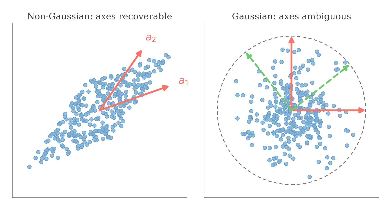
Non-Gaussian sources form an identifiable parallelogram while Gaussian sources form a rotationally symmetric cloud — Non-Gaussian sources contain directional structure that can reveal the mixing directions. A Gaussian subspace is rotationally symmetric, so different rotations cannot be distinguished.

The likelihood above also assumes that the observations are IID.

If observations have important temporal dependence, as in time-series data, ICA requires additional modeling.