Let z be a latent variable such that, z∼N(0,I), and let θ be the collections of weights of a neural network g(z;θ) that maps z∈Rk to Rd.
Also, let x given z follow a normal distribution x∣z∼N(g(z;θ),σ2I). We can find this distribution using an Expectation Maximization Algorithm.
Note that for Gaussian Mixture Models, the optimal choice of Q(z)=p(z∣x;θ) and we found it using Bayes' rule. We were able to do so because z was discrete and could take only k values.
However, for more complex models like the Variational Autoencoder, z is continuous. Therefore, it is intractable to compute p(z∣x;θ) explicitly. Instead, we will try to find an approximation of p(z∣x;θ).
Also note that we wanted to find Q(z)=p(z∣x;θ) so that our ELBO would be tight with logp(x;θ).
Since,
ELBO(x;Q,θ)=logp(x;θ)−DKL(Q∥pz∣x)
Therefore,
logp(x;θ)=ELBO(x;Q,θ)+DKL(Q∥pz∣x)
From this we can see that if we choose a Q(z) such that it maximizes our ELBO for a given value of θ, then our KL-divergence is minimized.
From this, we can find an approximate value for p(z∣x;θ) by choosing a Q from our family of distributions Q:
p(z∣x;θ)≈Q∈Qargmax(θmaxELBO(x;Q,θ))
We make a mean field assumption that assumes that Q(z) gives a distribution with independent coordinates which means that we can decompose Q(z) into Q1(z1)…Qk(zk).
Finally, we assume that Q is a normal distribution where the mean and variance come from the neural networks q(x;ϕ) and v(x;ψ) respectively. We set the covariance matrix to be a diagonal to enforce our mean field assumption. We can write this as:
Qi(z(i))=N(q(x(i);ϕ),diag(v(x(i);ψ))2)
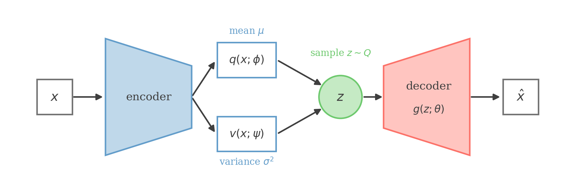
The encoder turns x into the parameters of Q — a mean q(x;ϕ) and a variance v(x;ψ); we sample a latent z∼Q and the decoder g(z;θ) maps it back to a reconstruction x^.
We use this Qi(z(i)) to find our ELBO for the M step.
Note that we no longer need the E step because we are directly using our Qi(z(i)). Therefore, instead of alternating maximization, we can use gradient ascent.
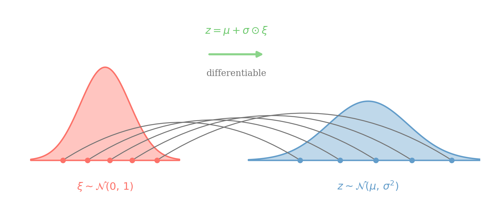
where z^(i) is just the reparameterized version of z(i) and z^(i)=q(x(i);ϕ)+v(x(i);ψ)⊙ξ(i)
Sampling z∼N(μ,σ2) is equivalent to drawing ξ∼N(0,1) and mapping z=μ+σ⊙ξ. Randomness lives in ξ, so gradients flow through μ and σ back to ϕ and ψ.
We can find all three derivatives by backpropagating through their respective neural networks.
p(x(i)∣z(i);θ) depends on the decoder neural network g(z(i);θ). And Qi(z(i)) depends on the encoder neural networks q(x(i);ϕ) and v(x(i);ψ).
Of course, since we still have an expectation, we will have to take multiple samples of z(i) in case of θ, and ξ(i) in case of ψ and ϕ and then take an average over the derivatives.
See derivation
See derivation
Please use a larger screen
This content is best viewed on a laptop or desktop device.